What it is
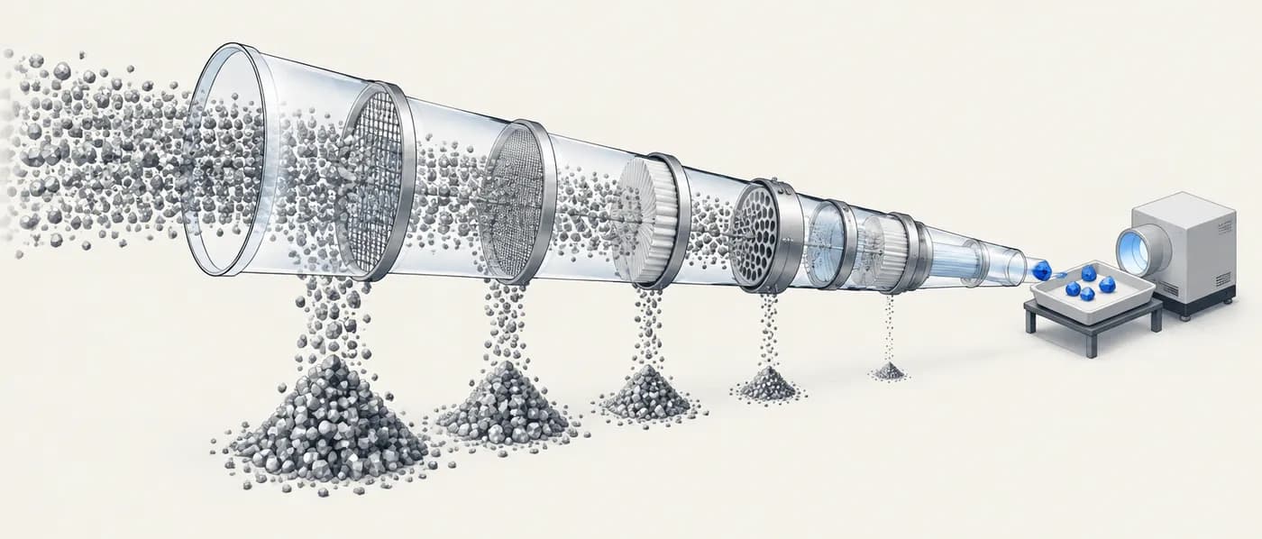
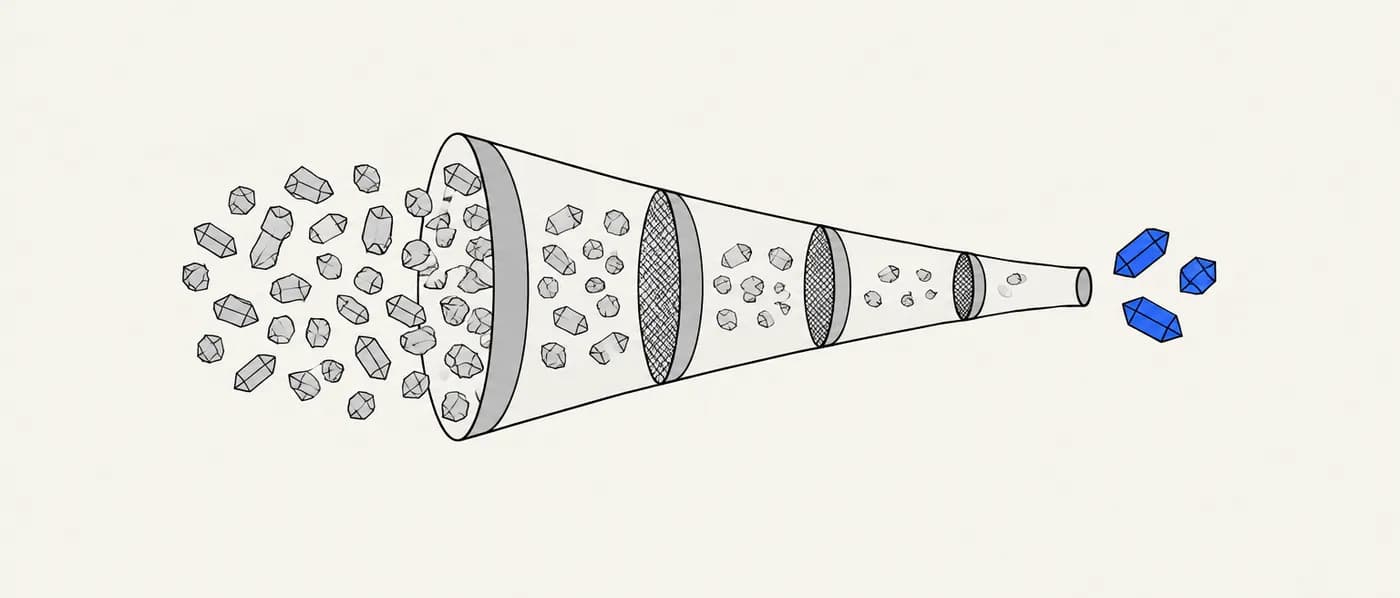
A screening funnel is the standard architecture of high-throughput materials discovery. You start from a large pool of candidate compositions or structures — often tens or hundreds of thousands drawn from databases such as Materials Project, OQMD, AFLOW or JARVIS — and pass them through a series of filters. Early filters are nearly free: element whitelists and blacklists, charge balance, a lookup of an already-computed property. Later filters are expensive: dedicated density functional theory (DFT) calculations, molecular dynamics, and finally synthesis and measurement. The output is a short list small enough to make in the lab.
The idea is older than computational materials science — pharmaceutical virtual screening and combinatorial chemistry used the same logic — but it became the backbone of the Materials Genome era once large DFT databases made property lookups instant. Curtarolo and co-workers described the pattern as a ‘high-throughput highway’: generate, compute, store, then filter with descriptors that capture the property you care about.
A funnel is not a single model or score. It is an ordered set of pass/fail (or ranked) decisions, each with a cost per candidate, a pass rate and an error rate. Designing a good funnel means choosing those three numbers deliberately rather than by accident.
Why it matters for R&D decisions
Compute, instrument time and synthesis capacity are the scarce resources in R&D. If an expensive step runs on candidates that a cheap rule could have eliminated, you pay for work that can never change the decision. A well-ordered funnel can cut the cost of a campaign by an order of magnitude while making the reasons for every rejection explicit — which matters when a manager, partner or investor asks why a material was or was not pursued.
The formula
Total cost = Σ_i (N_i × c_i), N_(i+1) = N_i × p_i, overall recall ≈ Π_i r_i
- N_i
- Number of candidates entering stage i
- c_i
- Cost per candidate at stage i (CPU-hours, instrument hours or money)
- p_i
- Pass rate of stage i (fraction kept)
- r_i
- Recall of stage i: fraction of truly good candidates the filter keeps
The recall product assumes filter errors are independent. Correlated errors (for example two filters that both rely on the same PBE calculation) can make the true loss larger or smaller.
How to apply it, step by step
- 1Define what ‘good’ means before filtering
Write the target as measurable criteria: e.g. ‘Li-ion conductivity above 1 mS/cm at room temperature, stable against Li metal or with a known interlayer, no Co, synthesisable below 1,000 °C’. Each criterion becomes a candidate filter. Criteria you cannot express as a filter belong in the final human review, not in the funnel.
- 2List possible filters with their cost and confidence
For each criterion, list the ways to test it — element rule, database lookup, machine-learning surrogate, dedicated DFT, simulation, experiment — and estimate the cost per candidate and how reliable each is. The same criterion often has a cheap, rough filter and an expensive, accurate one; use both, in that order.
- 3Order filters by cost, then by selectivity
Put the cheapest filters first. Between filters of similar cost, put the one that removes the most candidates first. Never run a filter that costs hours per candidate before one that costs milliseconds, unless the cheap one is so unreliable that it would remove most of the good candidates.
- 4Set thresholds loose early, tight late
Early filters are approximations, so give them generous thresholds — for stability, many teams accept materials up to roughly 25–50 meV/atom above the convex hull rather than only those exactly on it. Tighten thresholds at the stages where the measurement is more accurate.
- 5Size the funnel before running it
Estimate how many candidates will enter each stage and multiply by cost. If the expensive stage would still receive thousands of candidates, add another cheap filter or a ranking step in front of it. If a stage passes almost everything, it is not doing useful work.
- 6Audit what you threw away
Run known good materials (positive controls) through the funnel. If a filter rejects a material that is already known to work, the threshold or the descriptor is wrong. Keep the rejection reason for every candidate so the decision can be revisited when data improves.
Worked examples
Sizing a solid-electrolyte funnel (hypothetical numbers)
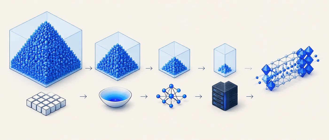
A team wants new lithium solid electrolytes and starts from 50,000 Li-containing structures in public DFT databases. All counts and costs below are hypothetical but of realistic order of magnitude.
- 01Stage 1 — element rules (no Co, no highly toxic or very scarce elements; cost ≈ 0): 50,000 → 8,000 candidates.
- 02Stage 2 — stability lookup, energy above hull ≤ 25 meV/atom (database lookup, cost ≈ 0): 8,000 → 1,500.
- 03Stage 3 — cheap conductivity proxy (structural descriptors or an ML model, seconds per candidate): 1,500 → 200.
- 04Stage 4 — nudged elastic band (NEB) Li-migration barriers at a hypothetical 500 CPU-hours per candidate: 200 × 500 = 100,000 CPU-hours.
- 05Counterfactual: running NEB directly on all 1,500 stable candidates would cost 1,500 × 500 = 750,000 CPU-hours — 7.5× more for the same final shortlist, if Stage 3 rarely discards good conductors.
The value of a cheap filter is set by the cost of the stage it protects, not by its own accuracy. Even a rough proxy pays for itself if it sits in front of an expensive step.
How false negatives compound across stages
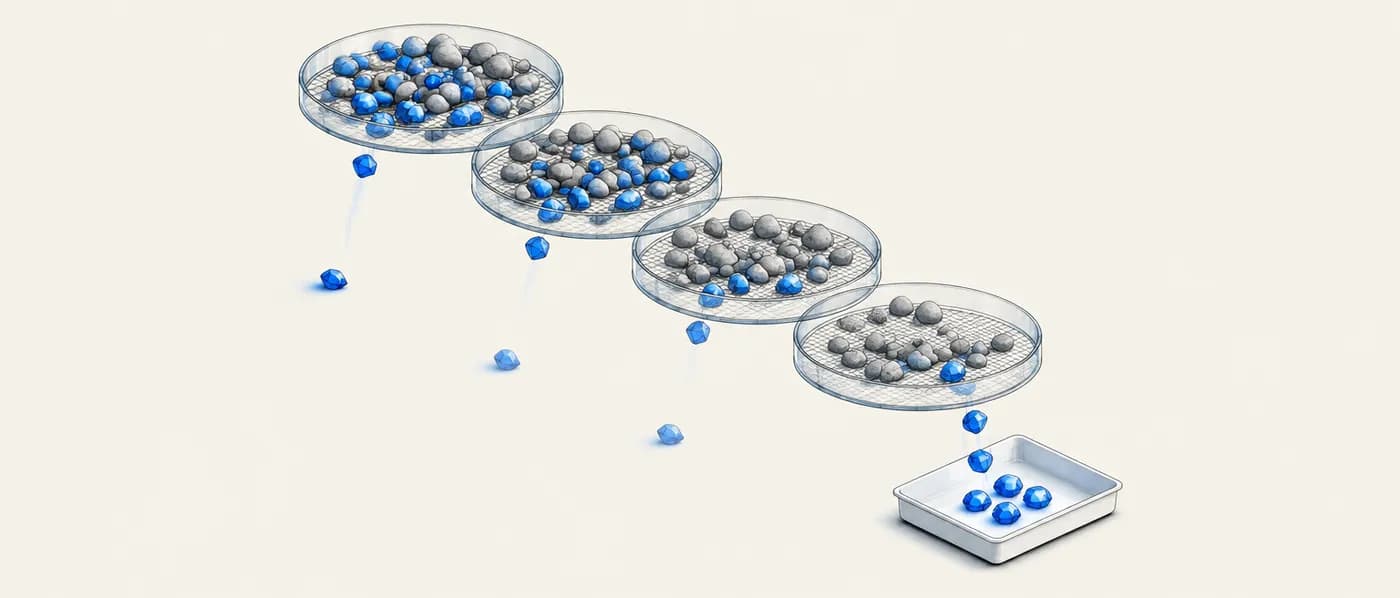
Each filter keeps most good candidates but not all. Suppose four sequential filters each have 90% recall (they keep 90% of the truly good materials) and their errors are independent.
- 01Overall recall = 0.90 × 0.90 × 0.90 × 0.90 = 0.9⁴ ≈ 0.656.
- 02So about one in three genuinely good materials is lost before reaching the lab.
- 03Loosening the two cheapest filters to 98% recall gives 0.98 × 0.98 × 0.90 × 0.90 ≈ 0.778.
- 04The cost: more candidates reach the expensive stages, so re-size the funnel (see the formula) to check the budget still holds.
Every added filter has a recall cost. Prefer fewer, well-validated filters over many marginal ones, and loosen the cheap filters first.
Catalyst screening: the hydrogen evolution example
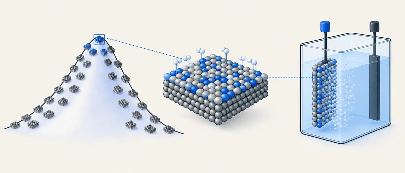
Greeley, Nørskov and co-workers (Nature Materials, 2006) screened binary surface alloys for the hydrogen evolution reaction (HER) computationally.
- 01Activity descriptor: the hydrogen adsorption free energy ΔG_H, computed with DFT; values near zero indicate high HER activity (the Sabatier principle).
- 02Stability descriptor: whether the solute stays in the surface layer under reaction conditions, also from DFT.
- 03Candidates were ranked on activity and filtered on stability, so only alloys that were both active and plausibly stable were proposed.
- 04A BiPt surface alloy was identified and then tested experimentally, with promising HER activity reported.
A funnel does not need many stages. Two well-chosen descriptors — one for performance, one for stability — are often enough to make a lab shortlist.
Typical stages and order-of-magnitude cost per candidate
| Stage | Typical tool | Cost per candidate (order of magnitude) | Typical role |
|---|---|---|---|
| Composition rules | Element lists, charge balance | Microseconds | Remove forbidden or impractical chemistries |
| Database lookup | Materials Project, OQMD, AFLOW, JARVIS | Milliseconds | Stability, band gap, density, known properties |
| ML surrogate | Trained property model | Milliseconds to seconds | Rank by predicted property |
| Standard DFT | Relaxation, static calculation | Tens to hundreds of CPU-hours | Confirm stability, compute missing properties |
| Advanced simulation | NEB, phonons, AIMD, hybrid functionals | Hundreds to thousands of CPU-hours | Transport, finite-temperature behaviour, accurate gaps |
| Synthesis and measurement | Lab work | Days to weeks of staff and instrument time | Ground truth |
When to use it — and when not to
- You have many more candidates than you can afford to compute or make in detail.
- The target can be broken into criteria that can each be tested at different cost and accuracy.
- You need an auditable record of why candidates were rejected.
- You are planning a computational campaign and need to estimate the compute budget up front.
- The candidate space is already small (a handful of compositions) — test them directly.
- There is no reasonable cheap proxy for the key property; a funnel with poor early filters mainly creates false negatives.
- The goal is to optimise a process for one chosen material — use design of experiments or Bayesian optimisation instead.
Common mistakes
Applying it in Lattice Graph
LatticeGraph’s search and filters act as the cheap front of the funnel: element constraints, stability and property thresholds across sources, with cross-source confidence showing where databases disagree before you spend compute or lab time.
- 01Express the hard constraints as search filters (elements included and excluded, stability tolerance, property ranges).
- 02Check the cross-source confidence of each surviving row; treat single-source values as provisional rather than as pass/fail.
- 03Shortlist the survivors and carry them into an application workflow (for example batteries or catalysts) for the next stage.
- 04Export the shortlist with its filter values and sources so the rejection logic is documented in your evidence pack.
Frequently asked questions
How many stages should a funnel have?
Usually three to six. Fewer stages lose less recall; add a stage only when it protects a much more expensive step or removes a large fraction of candidates for a defensible reason.
Should I rank or filter at each stage?
Use hard filters for true constraints (forbidden elements, safety). Use ranking when the descriptor is approximate, then take the top N forward. Ranking avoids discarding a candidate because it narrowly missed an uncertain threshold.
Can machine-learning models replace the early stages?
They can act as a fast filter or ranker, but check their error on chemistries like yours. If the model’s error is larger than the margin you are filtering on, it will mostly add noise.
References & further reading
- [1]Curtarolo, S. et al. (2013). The high-throughput highway to computational materials design. Nature Materials 12, 191–201.Overview of the generate–compute–store–filter pattern.
- [2]Jain, A. et al. (2013). Commentary: The Materials Project: A materials genome approach to accelerating materials innovation. APL Materials 1, 011002.The database that made instant property lookups routine.
- [3]Greeley, J., Jaramillo, T. F., Bonde, J., Chorkendorff, I. & Nørskov, J. K. (2006). Computational high-throughput screening of electrocatalytic materials for hydrogen evolution. Nature Materials 5, 909–913.Two-descriptor catalyst funnel with experimental follow-up.
- [4]Sendek, A. D. et al. (2017). Holistic computational structure screening of more than 12,000 candidates for solid lithium-ion conductor materials. Energy & Environmental Science 10, 306–320.A multi-stage solid-electrolyte funnel combining stability, electronic and ML conductivity filters.
- [5]Pyzer-Knapp, E. O., Suh, C., Gómez-Bombarelli, R., Aguilera-Iparraguirre, J. & Aspuru-Guzik, A. (2015). What is high-throughput virtual screening? A perspective from organic materials discovery. Annual Review of Materials Research 45, 195–216.Funnel design for molecular materials.