What it is
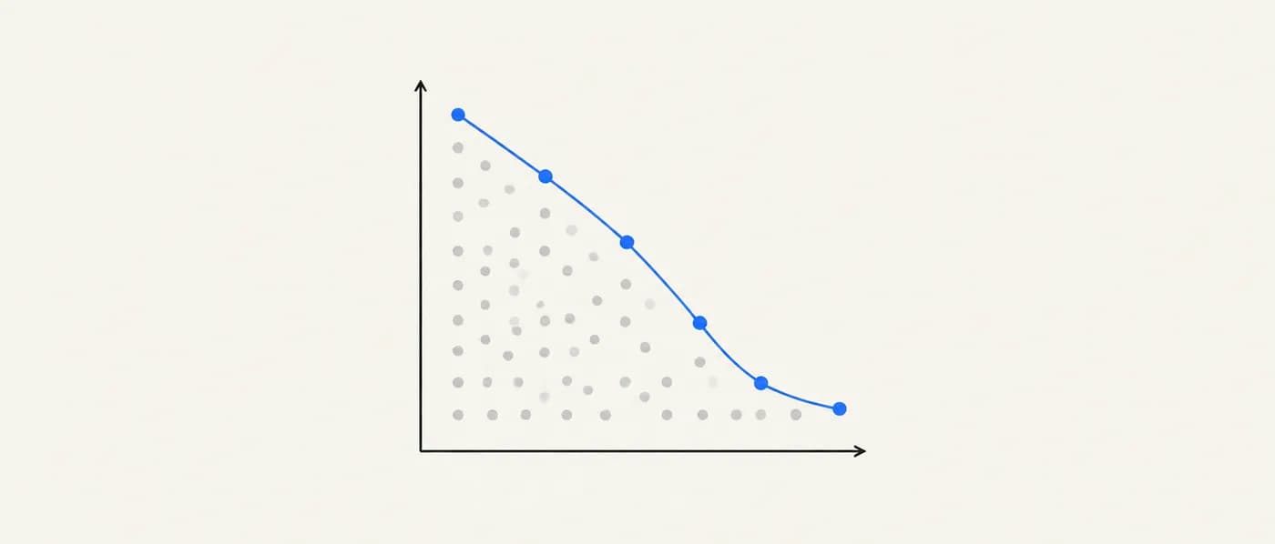
A Pareto front (also called a Pareto frontier or trade-off surface) is the set of non-dominated options in a problem with two or more objectives. The concept is named after the economist Vilfredo Pareto and is central to multi-objective optimisation. One option dominates another if it is at least as good on every objective and strictly better on at least one. Options that no other option dominates form the front.
In materials work, objectives conflict all the time: higher energy density usually costs more or is less stable; higher catalytic activity often comes with lower durability; stronger alloys are often less ductile. Collapsing everything into a single score hides these trade-offs. The Pareto front keeps them visible and lets you separate two questions that are often confused: which options are objectively inferior (dominated), and which of the remaining options best fits our priorities.
Once the front is known, a decision still has to be made. That requires an exchange rate between objectives — how much extra cost one more unit of performance is worth. Ashby calls these exchange constants and combines objectives into a penalty (or value) function. Changing the exchange rate moves the preferred point along the front, which is a useful way to test how sensitive a decision is to assumptions.
Why it matters for R&D decisions
Weighted scores feel objective but bake in arbitrary weights, and small changes to those weights can flip a ranking without anyone noticing. A Pareto front removes the dominated options without any weighting at all, so the debate narrows to the handful of options that represent genuine trade-offs. It also makes visible when a candidate is excellent on one axis but mediocre elsewhere — exactly the candidate a single score tends to bury and a niche application might want.
The formula
For objectives f₁ … fₖ to be minimised, candidate a dominates candidate b if fᵢ(a) ≤ fᵢ(b) for every i, and fⱼ(a) < fⱼ(b) for at least one j.
The Pareto front is the set of candidates not dominated by any other.
Value function (to choose a point on the front): V = Σ αᵢ · fᵢ
- fᵢ
- Objective i, expressed so that lower is better (negate any objective you want to maximise)
- a, b
- Two candidates being compared
- αᵢ
- Exchange constant (weight) converting objective i into a common unit, such as cost
- V
- Combined penalty to minimise (or value to maximise, if signs are flipped)
Finding the front needs no weights. Weights are only needed to choose a single point from it.
How to apply it, step by step
- 1Pick two or three objectives
Choose the objectives that genuinely conflict and matter to the decision, such as energy density, cost and cycle life. More than three becomes hard to visualise and interpret; treat the rest as constraints if you can.
- 2Apply hard constraints first
Remove candidates that fail pass/fail requirements before building the front. A non-dominated candidate that violates a constraint is still not a candidate.
- 3Put every objective in the same direction
Decide whether you are minimising or maximising each objective, and convert consistently. Use the same conditions and data sources for every candidate so comparisons are fair.
- 4Remove dominated candidates
Compare candidates pairwise, or sort by one objective and sweep along it. Whatever survives is the front. Plot it — two objectives on a scatter plot are usually enough to see the shape of the trade-off.
- 5Account for uncertainty
If two candidates differ by less than the error in the data, treat them as tied. Candidates just behind the front may be on it once uncertainty is considered, so keep them in view.
- 6Choose with explicit exchange rates
Agree how much one objective is worth in units of another, compute a value for each front member, and test how the choice changes as the exchange rate varies.
Worked examples
Five cathode candidates: energy vs cost (hypothetical numbers)
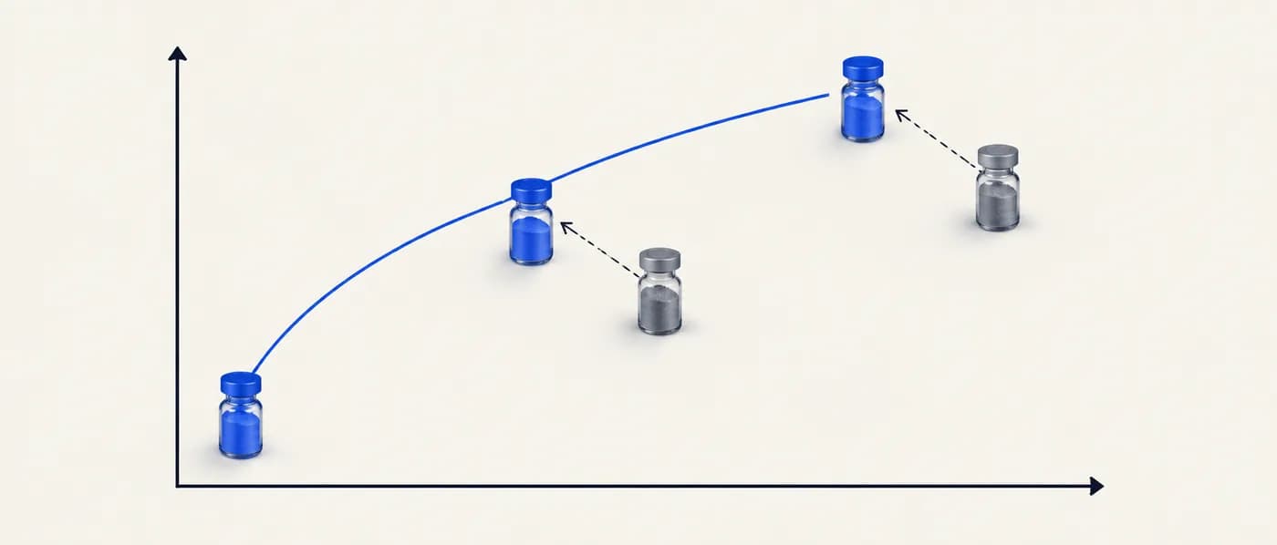
Objectives: maximise material-level specific energy (Wh/kg) and minimise material cost ($/kWh). The five candidates and their values are hypothetical, chosen to illustrate the method.
- 01A: 580 Wh/kg, $20/kWh · B: 700 Wh/kg, $35/kWh · C: 640 Wh/kg, $22/kWh · D: 600 Wh/kg, $30/kWh · E: 690 Wh/kg, $40/kWh.
- 02D vs C: C has more energy (640 > 600) and lower cost (22 < 30), so C dominates D.
- 03E vs B: B has more energy (700 > 690) and lower cost (35 < 40), so B dominates E.
- 04A: no candidate is cheaper than $20/kWh, so nothing dominates A.
- 05C: no candidate has ≥ 640 Wh/kg at ≤ $22/kWh other than C itself, so C is not dominated. B has the highest energy, so B is not dominated.
Two of five candidates were eliminated without any debate about priorities.
Choosing a point on the front with an exchange rate

Using the front from the previous example, value each candidate as V = α × energy − cost, where α ($/kWh per Wh/kg) expresses how much extra energy is worth. The α values are hypothetical.
- 01α = 0.1: A = 58 − 20 = 38; C = 64 − 22 = 42; B = 70 − 35 = 35 → C is preferred.
- 02α = 0.2: A = 116 − 20 = 96; C = 128 − 22 = 106; B = 140 − 35 = 105 → C is preferred, but only just.
- 03α = 0.3: A = 174 − 20 = 154; C = 192 − 22 = 170; B = 210 − 35 = 175 → B is preferred.
The choice hinges on the exchange rate, so agree it explicitly — and report how close the decision is to flipping.
Catalyst activity vs durability (hypothetical)
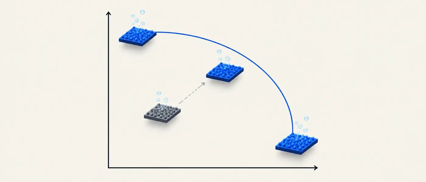
Four electrocatalyst candidates are compared on mass activity (higher is better) and activity retained after an accelerated stress test (higher is better). Values are hypothetical.
- 01P: activity 1.0, retention 90% · Q: 1.6, 60% · R: 1.3, 85% · S: 1.2, 70%.
- 02S vs R: R has higher activity (1.3 > 1.2) and higher retention (85% > 70%), so R dominates S.
- 03P has the highest retention, Q the highest activity; R is not beaten on both by either.
Knee points — where moving along the front costs a lot on one axis for little gain on the other — are often good default choices when exchange rates are uncertain.
When to use it — and when not to
- When two or three objectives conflict and stakeholders weigh them differently.
- Before building a weighted score, to remove options that are worse on every axis.
- When presenting a shortlist to decision-makers who need to see the trade-off, not just a winner.
- As the target of multi-objective optimisation or Bayesian optimisation campaigns.
- When a single objective clearly dominates the decision — rank by that objective after screening.
- With many objectives (more than about three or four), where almost every candidate becomes non-dominated; convert some objectives into constraints first.
- When the data uncertainty is larger than the differences between candidates — the front will not be meaningful until the data improves.
Common mistakes
Applying it in Lattice Graph
Use search to apply constraints, then compare the surviving candidates on two or three objectives side by side, with cross-source confidence telling you whether apparent differences are real.
- 01Filter candidates by hard constraints in materials search and shortlist the survivors.
- 02Compare shortlisted materials side by side on the objectives you care about (for battery work, the battery workflow gives voltage, theoretical capacity and related figures under the same assumptions).
- 03Check cross-source confidence for each objective; treat candidates whose differences fall within the spread between sources as tied.
- 04Record the non-dominated set and the exchange rate used to choose among it in your evidence pack.
Frequently asked questions
How is a Pareto front different from a weighted score?
A weighted score picks one winner using weights you choose. A Pareto front needs no weights; it identifies every option that is not beaten on all objectives at once. You still need weights to choose from the front, but you apply them to fewer, better options and can see how sensitive the choice is.
How many objectives can I use?
Two or three is practical. With more objectives, the proportion of non-dominated candidates grows quickly, so the front stops narrowing the field. Turn lower-priority objectives into constraints.
What is the “knee” of a Pareto front?
A region where small gains in one objective require large sacrifices in another. Knee points are often sensible compromises when exact exchange rates are unknown.
Can I use computed data to build a front?
Yes, but account for systematic errors. If a computed property has a typical error larger than the gap between two candidates, treat them as equivalent on that axis.
References & further reading
- [1]Ashby, M. F. (2000). Multi-objective optimization in material design and selection. Acta Materialia, 48(1), 359–369.Trade-off surfaces, exchange constants and penalty functions applied to materials selection.
- [2]Deb, K. (2001). Multi-Objective Optimization Using Evolutionary Algorithms. Wiley.Standard text on Pareto dominance and algorithms for finding fronts.
- [3]Miettinen, K. (1999). Nonlinear Multiobjective Optimization. Kluwer Academic Publishers.Mathematical treatment of Pareto optimality and methods for choosing among non-dominated solutions.
- [4]Ashby, M. F. (2017). Materials Selection in Mechanical Design, 5th edition. Butterworth-Heinemann (Elsevier).Chapters on multiple constraints and conflicting objectives.