Bottom-up cost modelling for new materials

What it is

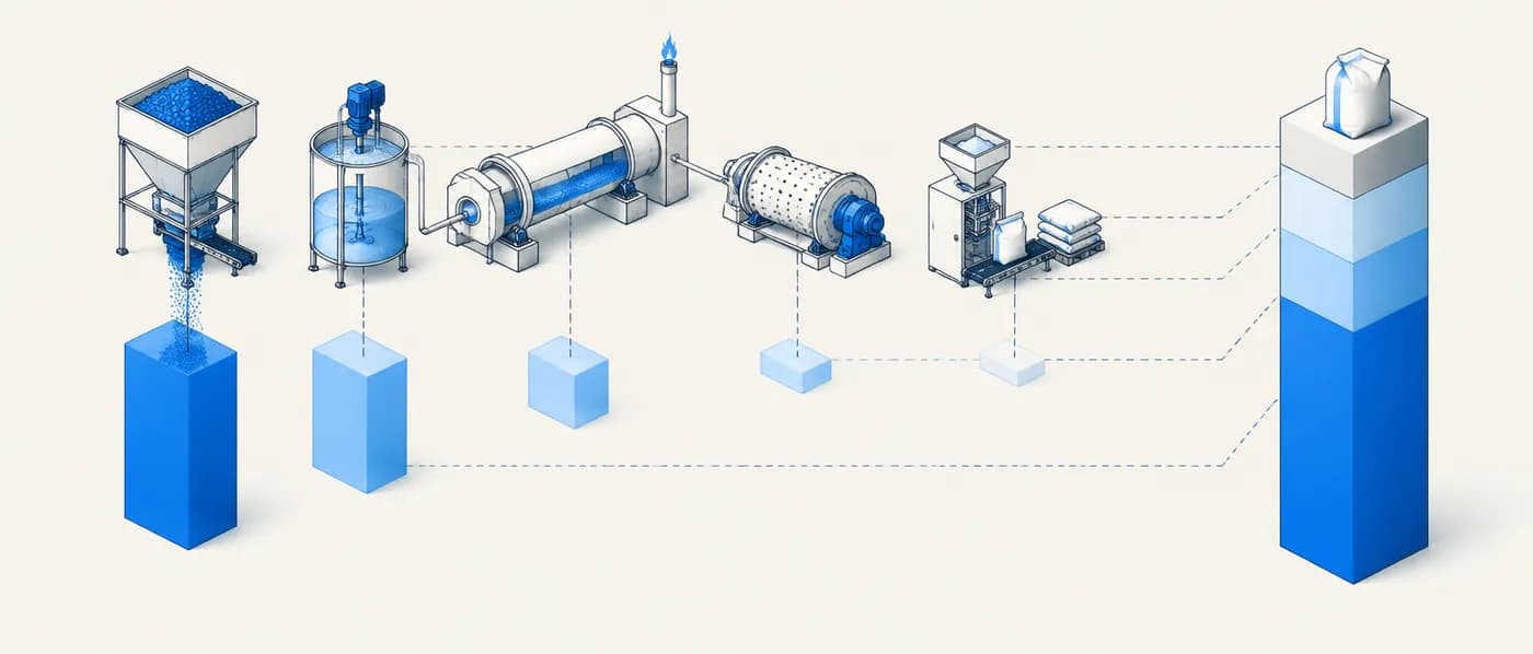
A bottom-up (process-based) cost model estimates the cost of making a material or device by modelling each process step: inputs consumed, equipment needed, throughput, energy, labour, yield and overhead. Instead of asking “what does the market charge?”, it asks “what would it cost to make this, at this scale, with this process?”

The approach is standard in engineering economics and has been formalised for materials as process-based cost modelling, notably by groups at MIT. In batteries, Argonne National Laboratory’s BatPaC model is a widely used public example. It estimates cell and pack cost from cell design, materials and manufacturing parameters.

For R&D, a cost model is most useful early, when it can still change design choices. Even a rough model shows which parameters dominate cost (often yield, cycle time or an expensive precursor) and sets cost targets for the research programme.

Schematic diagram: Bottom-up cost model — At a glance: Bottom-up cost model. Schematic, not to scale.

Why it matters for R&D decisions

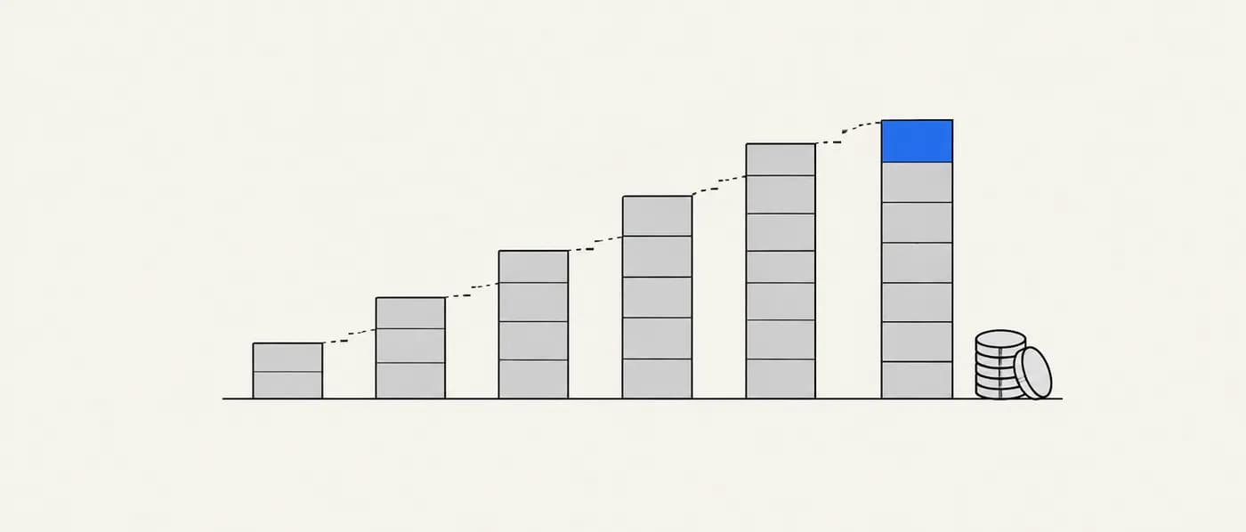
Many promising materials fail commercially on cost, not performance. A bottom-up model reveals that before scale-up: an inexpensive element in a slow, low-yield, high-temperature process can be expensive, and a pricier element in a fast, high-yield process can be cheap per unit of function. Making these trade-offs explicit lets teams set measurable R&D targets (for example, “raise yield from 85% to 95%”) and present credible cost cases at stage gates.

The formula

C = Σ (Pₘ × qₘ) ÷ Y  +  (CRF × K + L + E + O) ÷ Q      with  CRF = i(1+i)ⁿ ÷ ((1+i)ⁿ − 1)

C: Cost per kg of good product.
Pₘ, qₘ: Price per kg and quantity per kg of product for each raw material m (at 100% yield).
Y: Overall yield (fraction of input that ends up as saleable product).
K: Installed capital cost of the line.
CRF: Capital recovery factor: converts capital into an equivalent annual cost at interest rate i over n years.
L, E, O: Annual labour, energy and overhead costs.
Q: Annual output of good product (kg/year).

Real models split this per process step and add consumables, maintenance and scrap credits. The structure is the same.

How to apply it, step by step

1
Draw the process flow
List every step from raw materials to finished product: mixing, reaction, calcination, milling, coating, drying, packaging. Use lab procedures and analogous industrial processes.
2
Quantify inputs per kg of product
For each step, record raw materials, solvents, energy, cycle time and yield. Convert to amounts per kg of good output.
3
Size the equipment and capital
Estimate throughput per line and the equipment needed. Price capital with vendor quotes, scaling rules or published models, and annualise it with a capital recovery factor.
4
Add labour, energy and overhead
Estimate operators per shift, energy per kg and overhead (maintenance, quality control, facilities) as annual costs, then divide by annual output.
5
Convert to cost per unit of function
Divide by the functional performance (kWh/kg for batteries, activity or lifetime for catalysts, area for coatings) so candidates are compared on what they deliver.
6
Run sensitivities
Vary yield, throughput, capital, prices and scale. A tornado chart of the biggest drivers is often the most useful output for R&D.

Worked examples

Example 1

Cathode material cost per kWh (hypothetical prices)

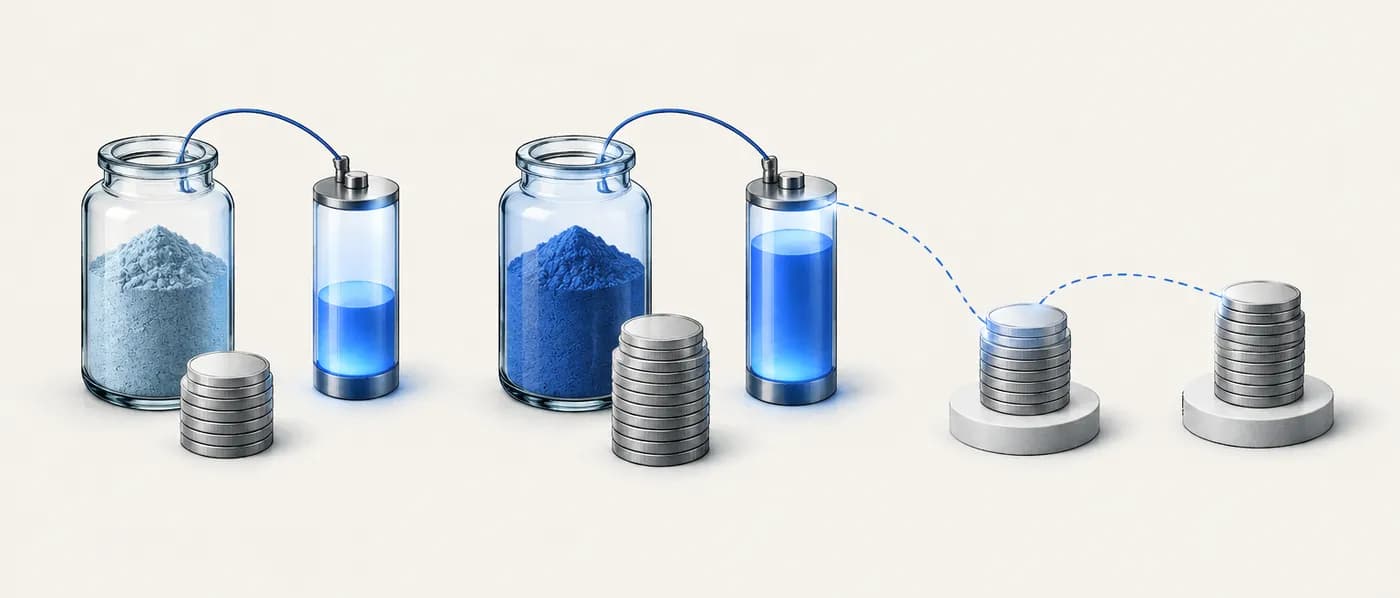
Two cathode materials with hypothetical prices. Energy is the material-level value: specific capacity × average voltage.

01Material A: $12/kg; 160 mAh/g at 3.3 V → 160 × 3.3 = 528 mWh/g = 0.528 kWh/kg.
02Cost per kWh for A = 12 ÷ 0.528 ≈ $22.7/kWh.
03Material B: $20/kg; 200 mAh/g at 3.7 V → 200 × 3.7 = 740 mWh/g = 0.740 kWh/kg.
04Cost per kWh for B = 20 ÷ 0.740 ≈ $27.0/kWh.

RESULTA is about 16% cheaper per kWh of cathode capacity, even though it stores 29% less energy per kg.

Compare cost per unit of function, not per kg. Also check cell-level effects: a lower-energy cathode needs more of every other cell component per kWh.

Example 2

Building up a cost per kg for a calcined powder (hypothetical)

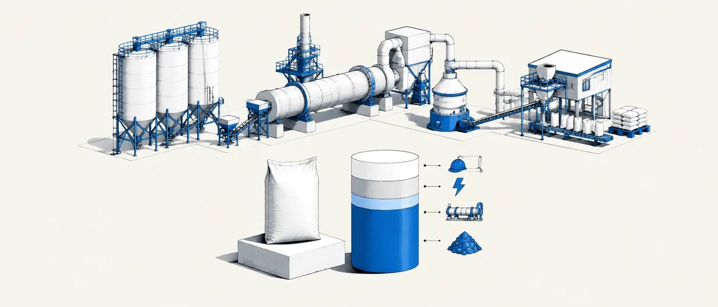
A hypothetical line making 5,000 t/year of good product. Installed capital $20M, 10-year life, 10% cost of capital.

01Capital recovery factor: (1.1)¹⁰ ≈ 2.594 → CRF = 0.1 × 2.594 ÷ (2.594 − 1) ≈ 0.163. Annual capital charge ≈ 0.163 × $20M ≈ $3.25M → ÷ 5,000,000 kg ≈ $0.65/kg.
02Energy: 5 kWh/kg × $0.08/kWh = $0.40/kg.
03Labour: $1.5M/year ÷ 5,000,000 kg = $0.30/kg.
04Raw materials: $8.00/kg at 100% yield; at 95% yield → 8.00 ÷ 0.95 ≈ $8.42/kg.
05Total ≈ 8.42 + 0.65 + 0.40 + 0.30 ≈ $9.77/kg (before overhead and margin).

RESULTRaw materials are ~86% of cost, so precursor choice and yield are the levers that matter most for this material.

The breakdown tells R&D where to work. If capital or energy had dominated, the priorities would be throughput and lower-temperature routes instead.

Example 3

Yield and learning: how fast costs can move

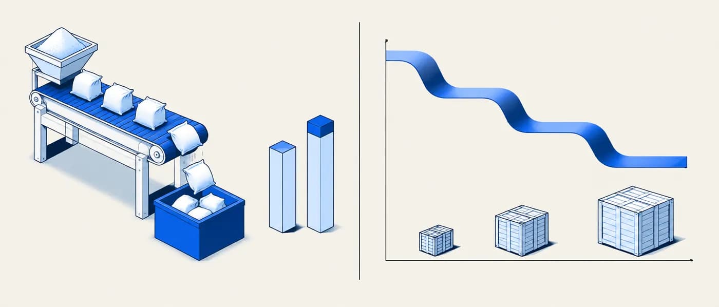
Two common sensitivities using the previous example.

01Yield drops from 95% to 85%: materials rise from 8.00 ÷ 0.95 ≈ $8.42 to 8.00 ÷ 0.85 ≈ $9.41/kg, an increase of about $1/kg (~10% of total cost), before accounting for lost throughput.
02Learning curve (Wright’s law): if cost falls 20% with each doubling of cumulative output, three doublings give 0.8³ ≈ 0.51 of the starting cost.
03Use both in the model: a near-term yield target for R&D, and a learning assumption (clearly labelled) for long-term projections.

RESULTA ten-point yield loss adds ~10% to cost. Learning effects can roughly halve cost over a few doublings of volume, if the assumed rate holds.

Yield is an R&D target you control now. Learning rates are assumptions: show them as scenarios, not forecasts.

Typical cost drivers and the R&D lever for each

Driver	Shows up as	R&D lever
Precursor price	High raw-material share	Alternative precursors, cheaper elements, less excess reagent
Yield / scrap	Materials ÷ Y grows	Process control, fewer steps, recycling of off-spec material
Cycle time	Low throughput Q → high capital per kg	Faster reactions, continuous processing
Process temperature	Energy and furnace capital	Lower-temperature or shorter calcination routes
Atmosphere / solvents	Consumables and safety capital	Air-stable chemistry, water-based processing, solvent recovery

When to use it — and when not to

Use it when

Before scale-up, to check whether a candidate can meet a cost target at volume.
Comparing synthesis routes for the same material.
Setting quantitative R&D targets (yield, cycle time, temperature) from cost sensitivities.
Preparing a cost case for a stage gate, partner or investor.

Don’t rely on it when

As a price forecast. Market prices also reflect margins, supply–demand balance and policy.
With capital and throughput guesses that are unanchored. Show ranges, or use a published model as a starting point.
To compare candidates per kg when they deliver different functional performance.

Common mistakes

Pricing only the raw materials.

Include yield, capital, energy, labour and overhead. For many advanced materials, processing is a large share of cost.

Comparing $/kg across materials with different performance.

Convert to cost per unit of function, such as $/kWh, before comparing.

Using lab yields and cycle times at production scale.

Estimate scaled values, label them as assumptions and test the sensitivity.

Hiding assumptions.

Publish the input table (prices with dates, scale, interest rate, equipment life) with the result so it can be challenged.

Ignoring cell- or system-level knock-on effects.

A cheaper but lower-energy material can raise the cost of everything else per kWh. Check at the level the customer buys.

Applying it in Lattice Graph

Use LatticeGraph to pull together the inputs a cost model needs (composition, synthesis route, performance and supply context) for each shortlisted candidate, and to keep the model’s assumptions with the evidence.

01Shortlist candidates and use the battery or other application workflow to get functional performance (for example, specific capacity in mAh/g and voltage from battery datasets) for the cost-per-function conversion.
02Pull synthesis recipes for each candidate to draft the process flow: precursors, steps and temperatures.
03Add element-level supply context to flag inputs whose price is exposed to concentration or criticality.
04Record the cost model inputs, sensitivities and resulting $/unit of function in your evidence pack.

DATASETS

Synthesis recipes (MatSyn25)Materials ProjectElements tableUSGS MRDS (Mineral Resources Data System)

Frequently asked questions

How accurate is a bottom-up model at the R&D stage?

Expect wide ranges early on. AACE International’s Class 5 (concept-screening) estimates carry accuracy ranges of roughly −20% to −50% on the low side and +30% to +100% on the high side. The value is in relative comparisons and identifying cost drivers, which are usually robust even when absolute numbers are uncertain.

What is BatPaC?

BatPaC is Argonne National Laboratory’s Battery Performance and Cost model, a publicly available spreadsheet that estimates lithium-ion cell and pack cost from design and manufacturing parameters. It is a good template for battery-material cost cases.

Should I include margin?

Model manufacturing cost first, then add margin separately if you need a price estimate. Keep the two distinct so cost drivers stay visible.

How do I pick the interest rate and equipment life?

Use your organisation’s cost of capital and typical equipment depreciation lives. Common illustrative values are 8–12% and 7–15 years. State them and test the sensitivity.

References & further reading

[1]
Nelson, P. A., Ahmed, S., Gallagher, K. G., & Dees, D. W. (2019). Modeling the Performance and Cost of Lithium-Ion Batteries for Electric-Drive Vehicles, Third Edition. Argonne National Laboratory, ANL/CSE-19/2.
Documentation for BatPaC, a public bottom-up battery cost model.
[2]
Field, F., Kirchain, R., & Roth, R. (2007). Process cost modeling: Strategic engineering and economic evaluation of materials technologies. JOM, 59(10), 21–32.
Process-based cost modelling for materials.
[3]
Wright, T. P. (1936). Factors Affecting the Cost of Airplanes. Journal of the Aeronautical Sciences, 3(4), 122–128.
Origin of the learning-curve relationship (Wright’s law).
[4]
Peters, M. S., Timmerhaus, K. D., & West, R. E. (2003). Plant Design and Economics for Chemical Engineers (5th ed.). McGraw-Hill.
Standard reference for capital estimation and capital recovery.