What it is
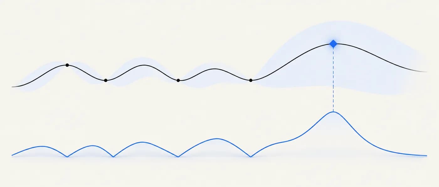
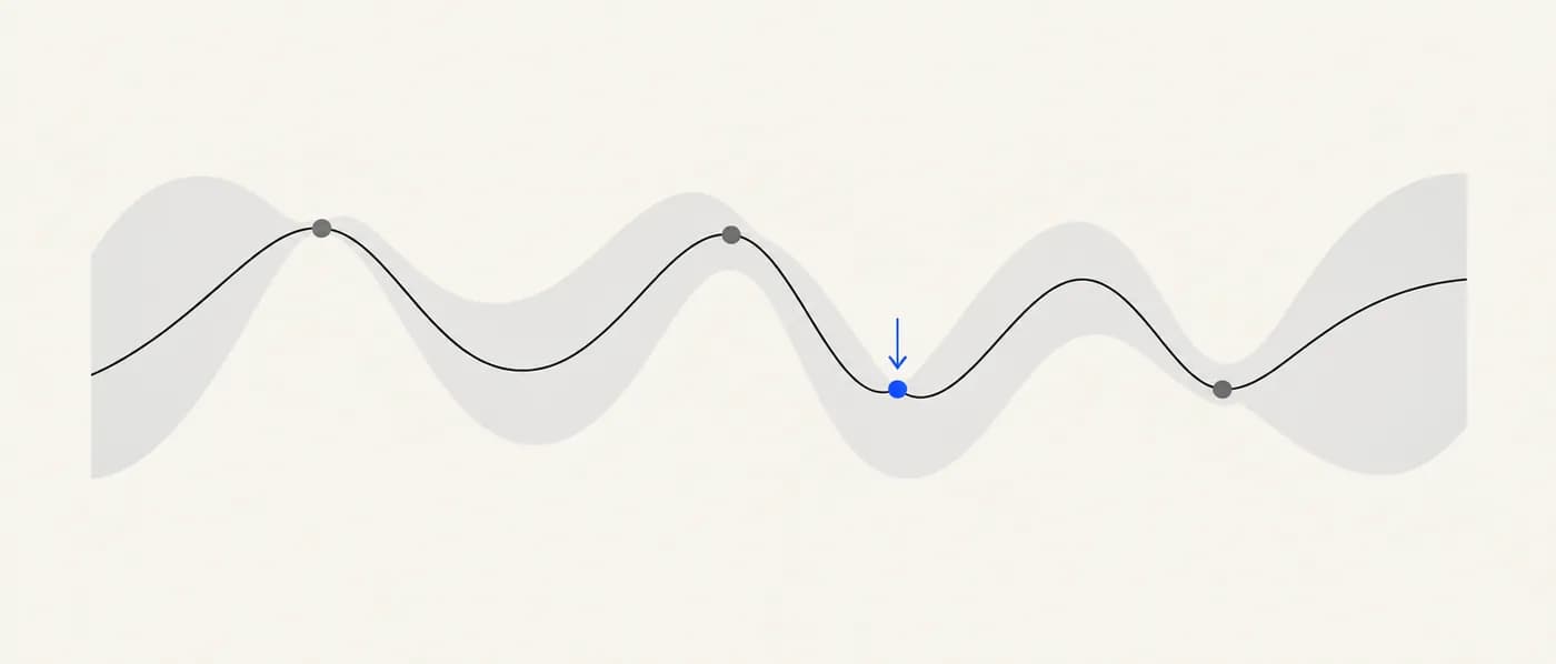
Bayesian optimisation (BO) is a strategy for optimising an expensive ‘black-box’ function — one you can only evaluate by running an experiment or a costly simulation. It keeps a probabilistic surrogate model of the response, typically a Gaussian process, that gives both a predicted value and an uncertainty at every untested point. After each new result, the model is updated.
An acquisition function then decides where to sample next. Expected improvement (EI), popularised by Jones, Schonlau and Welch in 1998, scores each candidate by how much it is expected to beat the best result so far, counting both its predicted value and its uncertainty. Upper confidence bound (UCB) and probability of improvement are common alternatives. This balance is called exploration (sampling uncertain regions) versus exploitation (sampling near the current best).
Active learning is the broader idea of choosing which data to collect next to improve a model or reach a goal fastest. In materials science, BO and active learning drive ‘self-driving labs’ such as the Ada platform for thin-film materials (MacLeod et al., 2020) and the mobile robotic chemist that optimised photocatalyst formulations (Burger et al., 2020).
Why it matters for R&D decisions
When each experiment costs a day of furnace time, a week of cell cycling or thousands of CPU-hours, the number of runs is the real budget. BO typically reaches good settings in fewer runs than grid searches or one-factor-at-a-time studies for problems with a handful of continuous variables, and it makes the reason for each next experiment explicit. It also works with existing data, so a campaign does not have to start from zero.
The formula
EI(x) = (μ(x) − f* − ξ) · Φ(Z) + σ(x) · φ(Z), Z = (μ(x) − f* − ξ) / σ(x); UCB(x) = μ(x) + κ · σ(x)
- μ(x), σ(x)
- Surrogate model’s predicted mean and standard deviation at candidate x
- f*
- Best value observed so far (for maximisation)
- ξ
- Small optional margin that encourages exploration (often 0–0.01, typically on a normalised response scale)
- Φ, φ
- Standard normal cumulative distribution and density functions
- κ
- UCB exploration weight; larger values favour uncertain regions
EI is zero where σ = 0 and the prediction does not beat f*. For minimisation, swap the sign of the improvement term.
How to apply it, step by step
- 1Define the objective and the variables
Choose one measurable objective to maximise or minimise (or a weighted combination), and a small set of continuous or discrete variables with sensible bounds — typically 2 to about 10. Fix everything else.
- 2Encode hard constraints
Exclude unsafe or impossible settings explicitly (maximum furnace temperature, solubility limits, composition sums to 1). An optimiser will happily propose a setting you cannot or should not run if you do not forbid it.
- 3Seed with initial data
Start with existing results or a small space-filling design (for example Latin hypercube or a small factorial) — often around 5–10 runs, or roughly two runs per variable. Literature and database values can inform priors and bounds.
- 4Iterate: fit, propose, run, update
Fit the surrogate, compute the acquisition function over the space, run the proposed experiment, add the result and repeat. Batch variants propose several experiments at once when parallel runs are possible.
- 5Decide when to stop and confirm
Stop when the expected improvement becomes small, the budget is spent, or a target is met. Replicate the best settings to make sure the optimum is real and not a noisy outlier.
Worked examples
Choosing the next run with expected improvement (hypothetical numbers)

Optimising room-temperature ionic conductivity. Best result so far f* = 1.0 mS/cm. The model offers two candidates. A: μ = 1.1, σ = 0.05 mS/cm (well understood, slightly better). B: μ = 0.9, σ = 0.4 mS/cm (poorly understood). Use ξ = 0.
- 01Candidate A: Z = (1.1 − 1.0)/0.05 = 2.0. Φ(2.0) ≈ 0.977, φ(2.0) ≈ 0.054. EI = 0.1 × 0.977 + 0.05 × 0.054 ≈ 0.098 + 0.003 = 0.100.
- 02Candidate B: Z = (0.9 − 1.0)/0.4 = −0.25. Φ(−0.25) ≈ 0.401, φ(−0.25) ≈ 0.387. EI = −0.1 × 0.401 + 0.4 × 0.387 ≈ −0.040 + 0.155 = 0.115.
- 03EI prefers B (0.115 > 0.100) even though its predicted mean is lower, because its large uncertainty leaves a real chance of a big improvement.
- 04With UCB and κ = 2: A = 1.1 + 2 × 0.05 = 1.2; B = 0.9 + 2 × 0.4 = 1.7, so UCB prefers B more strongly.
BO deliberately spends some runs on uncertainty. If you only ever test the highest prediction, you can get stuck near a local optimum.
Self-driving lab for thin films (Ada)
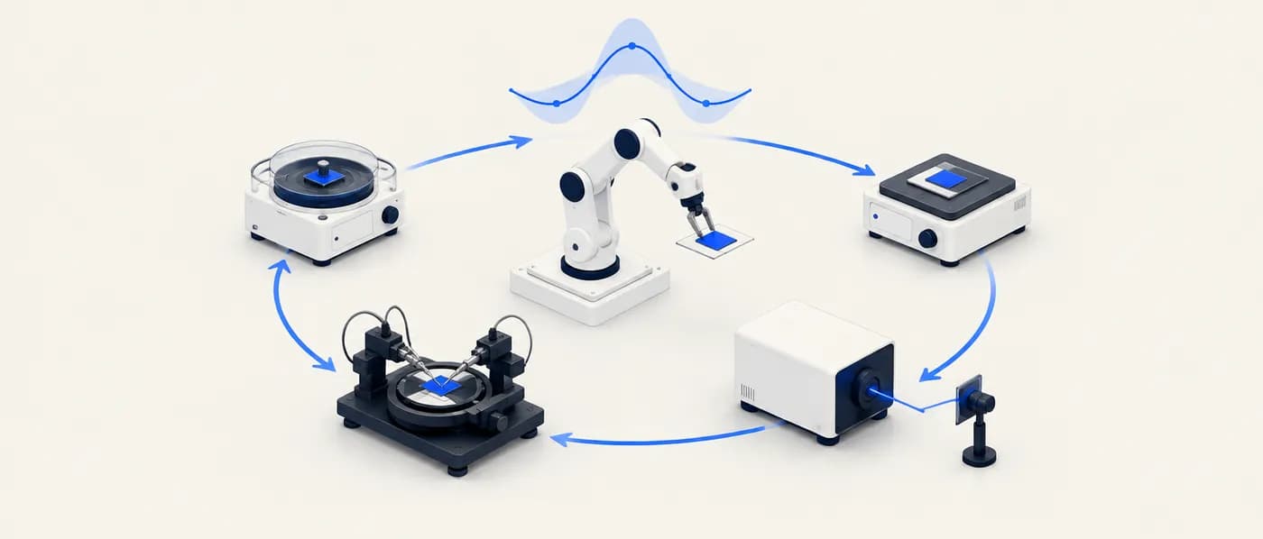
MacLeod and co-workers (Science Advances, 2020) built an autonomous platform that made and characterised thin films of an organic hole-transport material with dopant additives.
- 01Variables: processing and composition parameters such as dopant ratio and annealing time.
- 02Objective: a measure of hole mobility derived from optical and electrical measurements.
- 03Loop: a robot prepared films, measured them, and a Bayesian optimiser chose the next conditions.
- 04The platform ran many cycles autonomously and identified favourable conditions within its search space.
BO is most powerful when paired with automation, but the same loop works with a human running each experiment.
Hypothetical budget comparison for a two-variable process
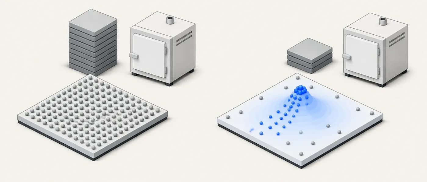
Tuning dopant fraction (0–10%) and sintering temperature (900–1,200 °C) for conductivity. Numbers are hypothetical.
- 01Grid search at 10 levels per variable: 10 × 10 = 100 runs.
- 02BO: seed with 10 space-filling runs, then 20 iterations: 10 + 20 = 30 runs.
- 03If each run costs two days of furnace and measurement time, the difference is (100 − 30) × 2 = 140 days of instrument time.
- 04The actual saving depends on how smooth the response is and how noisy the measurements are; it is not guaranteed.
Plan a BO budget up front and check progress; if the model is not improving after many runs, revisit variables, bounds or noise.
Common acquisition functions
| Acquisition | Idea | Tends to |
|---|---|---|
| Expected improvement (EI) | Expected amount by which a point beats the current best | Balanced default; widely used |
| Probability of improvement (PI) | Probability a point beats the current best (plus margin) | Exploit; can get stuck without a margin |
| Upper confidence bound (UCB) | Mean + κ × uncertainty | Explore more as κ increases |
| Thompson sampling | Optimise one random draw from the model | Natural batching and exploration |
| Expected hypervolume improvement | Improvement of a Pareto front | Multi-objective problems |
When to use it — and when not to
- Each experiment or simulation is expensive or slow.
- There are roughly 2–10 tunable variables with known bounds.
- The response is reasonably smooth and you can measure it repeatably.
- You have some existing data to seed the model, or can afford a small initial design.
- Experiments are cheap and fast — a grid or factorial design is simpler and gives a full map.
- You need to understand effects and interactions for a report or process transfer — DoE is more interpretable.
- Very high-dimensional or highly categorical spaces (thousands of compositions) without a good representation — use a screening funnel first.
- The measurement is so noisy that differences between settings are not resolvable.
Common mistakes
Applying it in Lattice Graph
LatticeGraph does not run the optimiser for you, but it provides the prior knowledge that makes BO start warm: reported values, ranges and recipes for the material and its neighbours.
- 01Collect measured and computed values for the material and close analogues to set variable bounds and an initial model.
- 02Use reported synthesis conditions to define safe, realistic ranges for processing variables.
- 03Record each BO iteration’s settings and results with the material in your evidence pack so the campaign is reproducible.
Frequently asked questions
Do I need a Gaussian process?
No. Gaussian processes are the common default for small datasets, but random forests, Bayesian neural networks and ensembles are also used as surrogates, especially with categorical variables or more data.
How many runs will BO need?
It depends on the number of variables, the smoothness of the response and the noise. There is no guaranteed number; monitor the best value and expected improvement as the campaign proceeds.
Can BO handle several objectives at once?
Yes. Multi-objective BO targets the Pareto front, for example with expected hypervolume improvement, so you can trade off conductivity against cost or stability.
References & further reading
- [1]Jones, D. R., Schonlau, M. & Welch, W. J. (1998). Efficient global optimization of expensive black-box functions. Journal of Global Optimization 13, 455–492.Expected improvement and the EGO algorithm.
- [2]Shahriari, B., Swersky, K., Wang, Z., Adams, R. P. & de Freitas, N. (2016). Taking the human out of the loop: A review of Bayesian optimization. Proceedings of the IEEE 104, 148–175.Accessible review of surrogates and acquisition functions.
- [3]Rasmussen, C. E. & Williams, C. K. I. (2006). Gaussian Processes for Machine Learning. MIT Press.Standard reference on Gaussian processes.
- [4]MacLeod, B. P. et al. (2020). Self-driving laboratory for accelerated discovery of thin-film materials. Science Advances 6, eaaz8867.Ada self-driving lab using Bayesian optimisation.
- [5]Burger, B. et al. (2020). A mobile robotic chemist. Nature 583, 237–241.Autonomous search over photocatalyst formulations with Bayesian optimisation.
- [6]Lookman, T., Balachandran, P. V., Xue, D. & Yuan, R. (2019). Active learning in materials science with emphasis on adaptive sampling using uncertainties for targeted design. npj Computational Materials 5, 21.Review of active learning in materials.