What it is
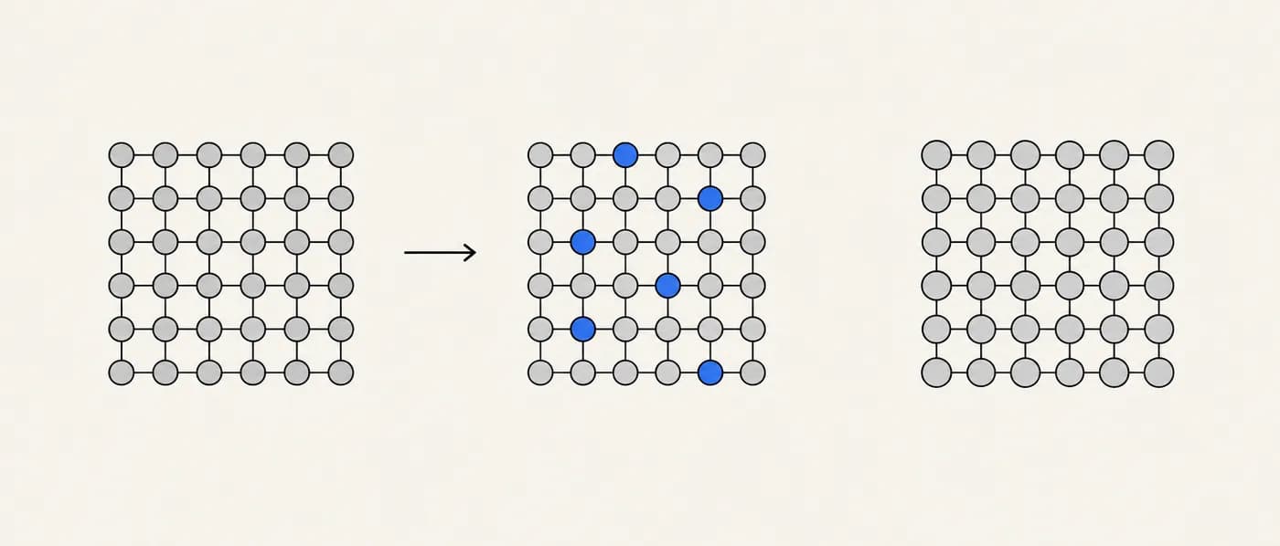
In the 1920s and 1930s William Hume-Rothery and co-workers studied why some metals mix freely while others barely dissolve in each other. From systematic measurements, especially on copper and silver alloys, they extracted a small set of empirical conditions for substitutional solid solutions — alloys in which solute atoms replace solvent atoms on the same lattice.
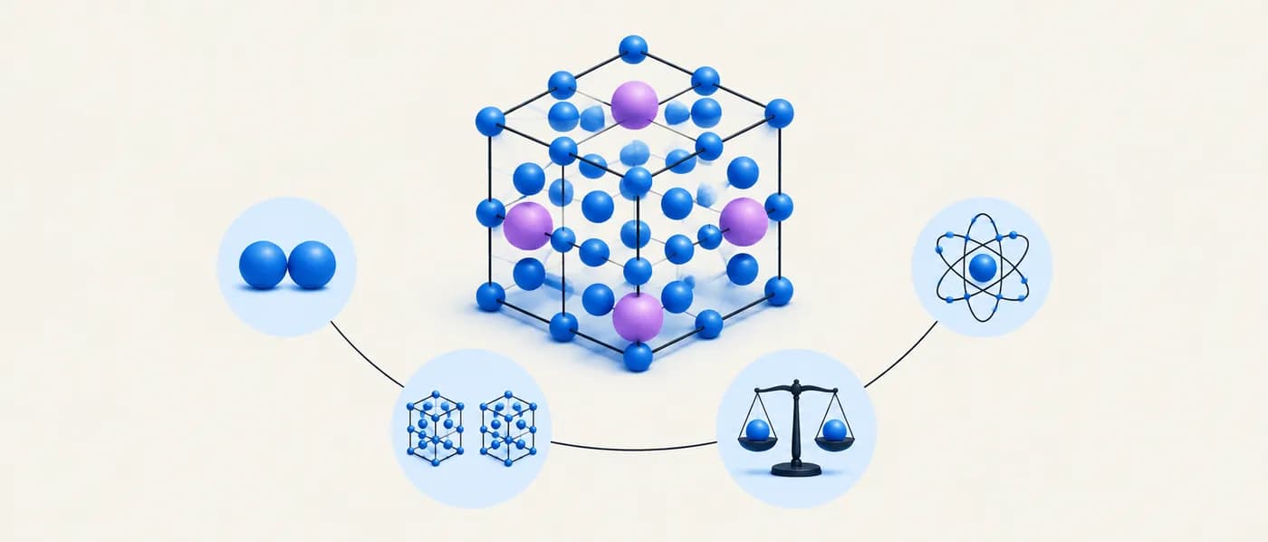
The rules are usually stated as four conditions. Size: the atomic radii of solute and solvent should differ by less than about 15%; beyond that, lattice strain limits solubility. Crystal structure: complete solubility across all compositions requires both elements to have the same crystal structure. Electronegativity: a large electronegativity difference favours the formation of intermetallic compounds over a solid solution. Valence: complete solubility requires similar valence, and a metal tends to dissolve a metal of higher valence more readily than one of lower valence.
Hume-Rothery also showed that some alloy phases form at characteristic valence-electron-to-atom ratios (e/a), the so-called electron compounds — for example β-brass near e/a = 3/2. Modern multi-component alloy design, including high-entropy alloys, still uses size-mismatch and electronegativity descriptors descended from these rules.
Why it matters for R&D decisions
Alloying and doping are among the most common ways to tune a material. Before computing or melting anything, the Hume-Rothery rules tell you whether a substitution is likely to dissolve into the host lattice, form a second phase, or create an intermetallic — which in turn determines strength, conductivity and corrosion behaviour.
The formula
Δr (%) = |r_solute − r_solvent| / r_solvent × 100 ; favourable if Δr ≲ 15%
- r_solute, r_solvent
- Atomic (metallic) radii, ideally for 12-fold coordination
- Δχ
- Electronegativity difference (Pauling scale); small values favour solid solutions
- e/a
- Average number of valence electrons per atom; governs electron-compound phase boundaries
Darken–Gurry maps plot electronegativity against atomic radius and draw an ellipse (commonly ±15% in radius and about ±0.4 in electronegativity) around the solvent; elements inside are candidates for extensive solubility.
How to apply it, step by step
- 1Identify solvent and solute
The solvent is the host metal (the majority element); the solute is the alloying element or dopant.
- 2Check the size factor
Compute Δr from consistent metallic radii (same coordination). Below ~15% is favourable; above it, expect limited solubility.
- 3Compare crystal structures
Same structure (for example both FCC) is required for complete solubility; different structures limit solubility at some composition.
- 4Compare electronegativity and valence
Small Δχ favours solid solution; large Δχ favours intermetallics. Similar valence favours wide solubility; higher-valence solutes dissolve more readily in lower-valence solvents than the reverse.
- 5Confirm with phase diagrams or calculations
Check an assessed phase diagram, CALPHAD model or DFT hull for the binary before relying on the prediction.
Worked examples
Cu–Ni: all four rules satisfied
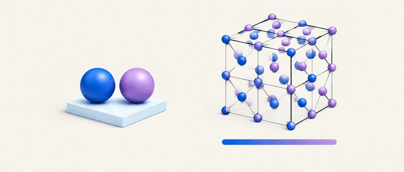
Approximate metallic radii (12-fold coordination): Cu 1.28 Å, Ni 1.25 Å. Both FCC. Pauling electronegativities: Cu 1.90, Ni 1.91.
- 01Size: Δr = |1.25 − 1.28| / 1.28 × 100 ≈ 2.3% — well under 15%.
- 02Structure: both FCC.
- 03Electronegativity: Δχ = 0.01 — negligible.
- 04Valence: similar for the purposes of the rule.
When every rule is comfortably satisfied, complete solubility is likely.
Cu–Ag: passing the rules isn’t enough
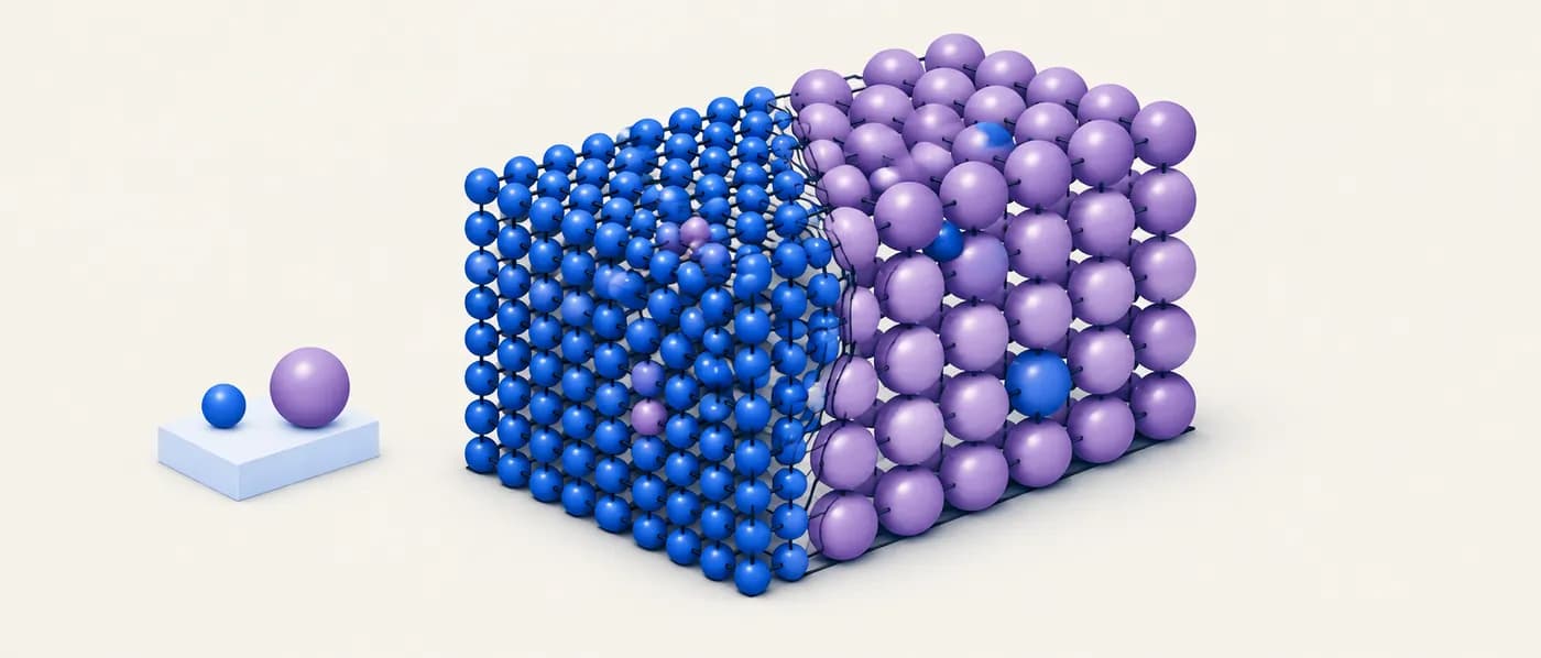
Metallic radii: Cu 1.28 Å, Ag 1.44 Å. Both FCC, both monovalent. Electronegativities: Cu 1.90, Ag 1.93.
- 01Size: Δr = |1.44 − 1.28| / 1.28 × 100 ≈ 12.5% — under 15%, but near the limit.
- 02Structure: both FCC.
- 03Electronegativity: Δχ = 0.03 — small.
- 04Valence: both 1.
Size mismatches in the 10–15% range already cost significant strain energy. Treat the 15% line as a soft boundary and confirm with the phase diagram.
Cu–Zn: valence and electron compounds
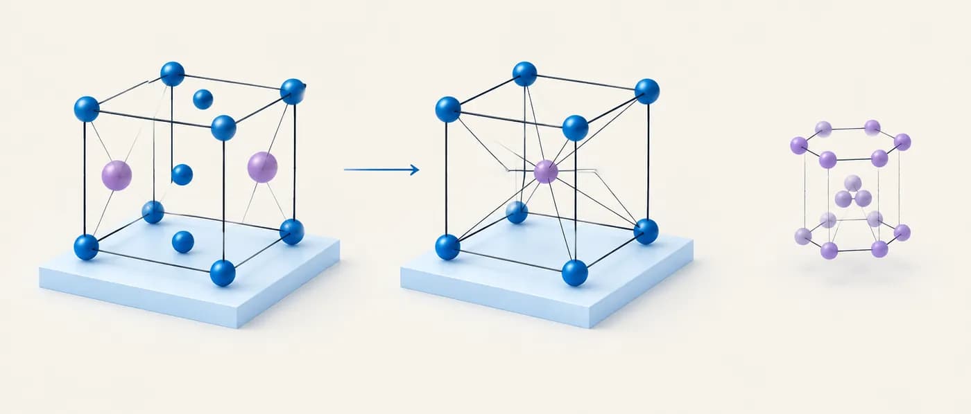
Metallic radii: Cu 1.28 Å, Zn 1.39 Å. Cu is FCC; Zn is HCP. Cu contributes ~1 valence electron, Zn ~2.
- 01Size: Δr = |1.39 − 1.28| / 1.28 × 100 ≈ 8.6% — favourable.
- 02Structure: different (FCC vs HCP), so complete solubility is not expected.
- 03Valence: Zn (higher valence) dissolves substantially in Cu — α-brass stays FCC up to roughly 35–38 wt% Zn.
- 04Beyond that, phases appear at characteristic electron-to-atom ratios: β-brass (CuZn) near e/a = 3/2 = 1.5.
Valence and e/a explain where solubility ends and which intermediate phases form — the basis of brass metallurgy.
Quick checklist
| Rule | Favourable | Unfavourable |
|---|---|---|
| Atomic size | Δr < ~15% | Δr > ~15%: limited solubility |
| Crystal structure | Same structure (needed for complete solubility) | Different structures: solubility ends at some composition |
| Electronegativity | Small Δχ | Large Δχ: intermetallic compounds favoured |
| Valence | Similar valence; higher-valence solute in lower-valence solvent | Lower-valence solute in higher-valence solvent: less soluble |
When to use it — and when not to
- First-pass screening of alloying additions and dopants in metals.
- Explaining why a binary system is isomorphous, eutectic or forms intermetallics.
- Choosing substitutions in multi-component alloys, alongside modern size-mismatch and mixing-enthalpy descriptors.
- Teaching and quick decisions in alloy development meetings.
- Ionic or covalent compounds — use Pauling’s rules or tolerance factors instead.
- Interstitial solid solutions (C, N, H in metals), which follow different size criteria.
- As a substitute for an assessed phase diagram when one exists.
Common mistakes
Applying it in Lattice Graph
LatticeGraph lets you check alloy and dopant ideas against computed binary and ternary stability data and known experimental structures.
- 01Search the binary or ternary system to see which ordered compounds and solid-solution end members are reported, and their hull distances.
- 02Compare the same phases across computed databases to judge confidence.
- 03Use elastic data where available to follow up with mechanical screens such as the Pugh ratio.
Frequently asked questions
Why 15%?
It is an empirical boundary from Hume-Rothery’s measurements: beyond roughly 15% size difference, solubility was found to be severely restricted because of lattice strain. It is not a sharp physical threshold.
Do the rules apply to high-entropy alloys?
Their spirit does. Researchers use an average atomic-size mismatch parameter and mixing enthalpy to predict single-phase solid solutions in multi-principal-element alloys, extending the size and electronegativity ideas.
What is an electron compound?
An intermetallic phase whose stability is tied to a characteristic ratio of valence electrons to atoms (e/a), such as β-brass near 3/2. Hume-Rothery identified these regularities in copper and silver alloys.
References & further reading
- [1]Hume-Rothery, W., Mabbott, G. W. & Channel-Evans, K. M. (1934). The freezing points, melting points, and solid solubility limits of the alloys of silver and copper with the elements of the B sub-groups. Philosophical Transactions of the Royal Society A 233, 1–97.Systematic data behind the size and valence rules.
- [2]Hume-Rothery, W. (1936). The Structure of Metals and Alloys. Institute of Metals, London.Classic monograph setting out the rules.
- [3]Darken, L. S. & Gurry, R. W. (1953). Physical Chemistry of Metals. McGraw-Hill.Electronegativity–radius maps for predicting solubility.
- [4]Zhang, Y., Zhou, Y. J., Lin, J. P., Chen, G. L. & Liaw, P. K. (2008). Solid-solution phase formation rules for multi-component alloys. Advanced Engineering Materials 10, 534–538.Size-mismatch and mixing-enthalpy criteria for high-entropy alloys.