Design of Experiments (DoE) for materials synthesis

What it is

Design of experiments (DoE) is a statistical approach to planning experiments so that each run carries as much information as possible. Its foundations were laid by Ronald Fisher in agricultural research in the 1920s and 1930s, and it was extended to industrial process optimisation by George Box and others, including the response-surface methods of Box and Wilson (1951). It is now standard practice in chemical, pharmaceutical and semiconductor process development.

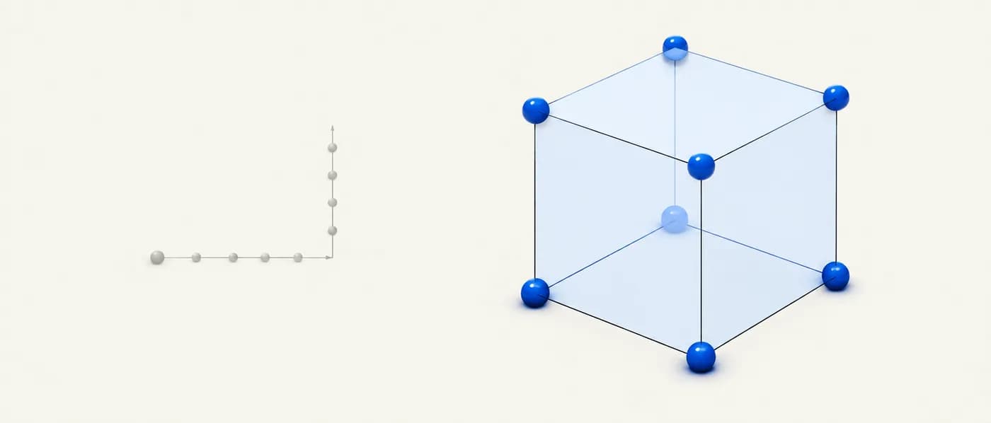
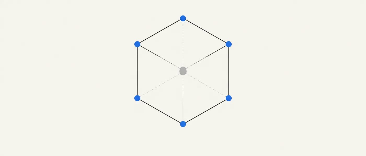
The core idea is to vary several factors at once according to a design matrix. In a two-level full factorial design, every factor is set to a ‘low’ and a ‘high’ level, and every combination is run: 2³ = 8 runs for three factors. From those eight runs you can estimate the main effect of each factor and every interaction between them. Changing one factor at a time (OFAT) from a baseline cannot detect interactions at all, and usually needs more runs to reach the same precision.

DoE is typically used in stages: a screening design to find which of many factors matter, then a more detailed design on the important few, and finally a response-surface design to locate the optimum and map the region around it.

Schematic diagram: Design of Experiments (DoE) — At a glance: Design of Experiments (DoE). Schematic, not to scale.

Why it matters for R&D decisions

Synthesis and processing outcomes in materials often depend on interactions: a longer dwell helps at low temperature but not at high temperature; a reducing atmosphere matters only above a certain temperature. If you only ever change one factor at a time, you will miss these, waste furnace time and may conclude a factor ‘does nothing’ when it matters strongly in another part of the space. DoE gives reliable conclusions from a fixed, planned budget of runs and makes the analysis reproducible.

The formula

Runs (full factorial) = 2^k;  Runs (fractional) = 2^(k−p);  Effect of A = ȳ(A high) − ȳ(A low);  Interaction AB = ȳ(AB sign +) − ȳ(AB sign −)

k: Number of factors, each tested at two levels
p: Number of generators used to fractionate the design (each halves the run count)
ȳ(A high): Mean response of all runs with factor A at its high level
AB sign: Product of the coded levels (−1/+1) of A and B in each run

With coded levels −1 and +1, an effect is the change in mean response when a factor moves from low to high. Regression coefficients are half the effects.

How to apply it, step by step

1
Fix the chemistry and define the response
DoE is for tuning conditions once you know which material you are making. Choose one or two measurable responses — phase purity from XRD, density, conductivity, capacity — and decide how they will be measured consistently.
2
Choose factors and realistic levels
List the factors you can control (temperature, time, atmosphere, precursor ratio, milling time, heating rate). Set low and high levels far enough apart to produce a visible effect but within safe, sensible limits — often informed by the analogue recipes you started from.
3
Pick a design that matches the goal and budget
Many factors and little prior knowledge: a fractional factorial or Plackett–Burman screening design. Three to five important factors: a full or high-resolution fractional factorial. Looking for an optimum or curvature: a central composite or Box–Behnken response-surface design.
4
Randomise, replicate and add centre points
Run in random order so drift (furnace ageing, humidity, precursor batch) is not confused with a factor. Add replicated centre points to estimate run-to-run noise and detect curvature.
5
Analyse effects, then confirm
Compute main effects and interactions, or fit a regression model. Judge effects against the noise estimated from replicates. Then run a confirmation experiment at the predicted best setting before adopting it.

Worked examples

Example 1

2³ factorial for a calcination step (hypothetical data)

Three factors for a cathode calcination: A = temperature (650 / 750 °C), B = time (4 / 12 h), C = atmosphere (Ar / 5% H₂ in Ar). Response = phase purity (%) from XRD. The eight results below are hypothetical. Coded runs (A, B, C) → purity: (−,−,−) 82 · (+,−,−) 94 · (−,+,−) 90 · (+,+,−) 95 · (−,−,+) 84 · (+,−,+) 96 · (−,+,+) 91 · (+,+,+) 97.

01Effect of A (temperature) = mean of high-A runs − mean of low-A runs = (94 + 95 + 96 + 97)/4 − (82 + 90 + 84 + 91)/4 = 95.5 − 86.75 = +8.75 points.
02Effect of B (time) = (90 + 95 + 91 + 97)/4 − (82 + 94 + 84 + 96)/4 = 93.25 − 89.0 = +4.25 points.
03Effect of C (atmosphere) = (84 + 96 + 91 + 97)/4 − (82 + 94 + 90 + 95)/4 = 92.0 − 90.25 = +1.75 points.
04AB interaction: runs with A×B = + are (−,−),(+,+): (82 + 95 + 84 + 97)/4 = 89.5; runs with A×B = − : (94 + 90 + 96 + 91)/4 = 92.75. AB = 89.5 − 92.75 = −3.25.
05Interpretation of AB: at 650 °C, longer time raises purity by (90 + 91)/2 − (82 + 84)/2 = 7.5 points; at 750 °C by only (95 + 97)/2 − (94 + 96)/2 = 1.0 point. Check: (1.0 − 7.5)/2 = −3.25.

RESULTTemperature matters most; time matters mainly at the lower temperature; atmosphere has a small effect. Running at 750 °C for 4 h gives nearly the same purity as 12 h, saving 8 hours per batch.

An OFAT study starting at 650 °C would have concluded that time is important; the factorial shows it hardly matters at the better temperature.

Example 2

Screening six factors with 16 runs

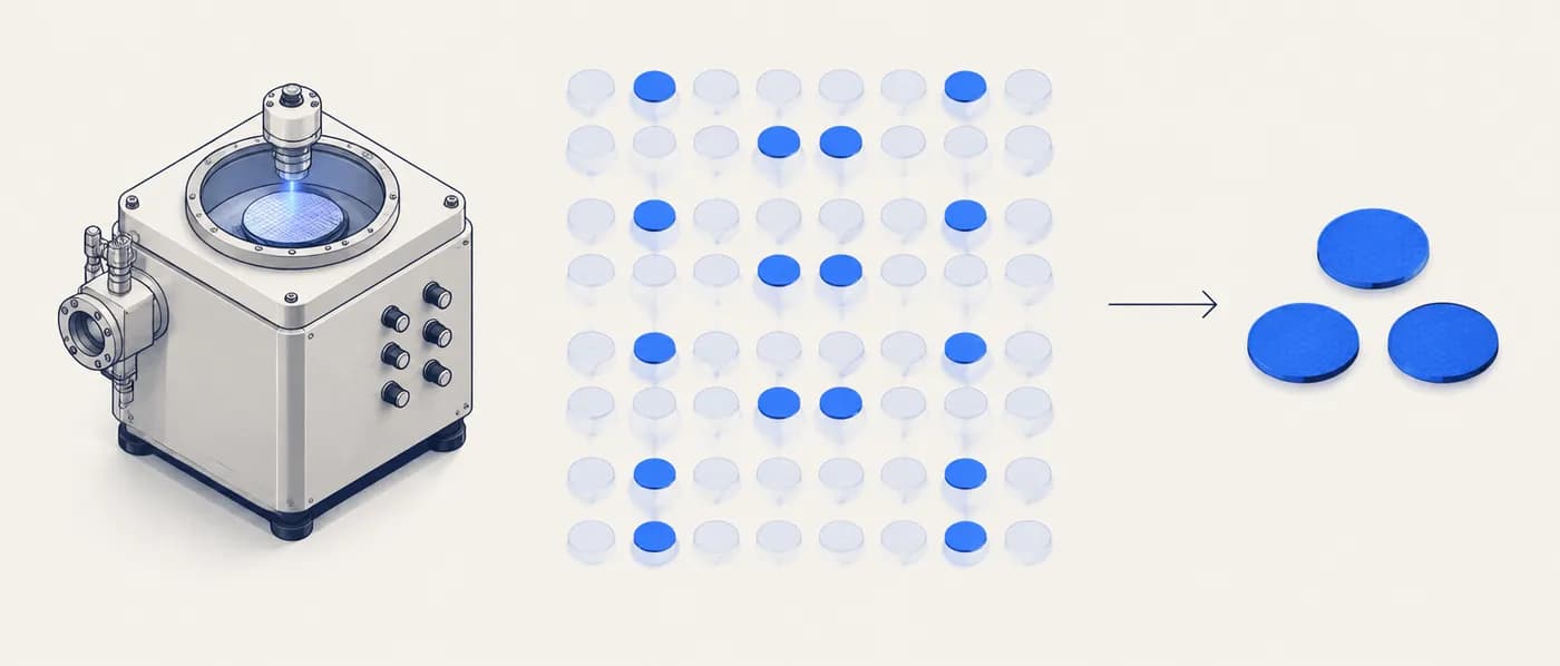
A thin-film deposition has six possibly important factors (substrate temperature, pressure, power, gas ratio, deposition time, anneal temperature).

01Full factorial: 2⁶ = 64 runs — too many.
02Fractional factorial 2^(6−2): 2⁴ = 16 runs, using generators such as E = ABC and F = BCD.
03This design has resolution IV: main effects are not confounded with each other or with two-factor interactions, though some two-factor interactions are confounded with each other.
04Analyse the 16 runs, identify the two or three dominant factors, then run a focused design on those.

RESULTThe important factors are found with a quarter of the full-factorial effort.

Screen first with a fractional design; spend detailed runs only on factors that matter.

Example 3

Finding an optimum with a central composite design

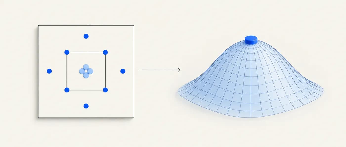
After screening, two factors remain important: sintering temperature and dopant fraction for a solid electrolyte; the response is ionic conductivity.

01A two-factor central composite design uses 4 factorial points + 4 axial (star) points + centre points.
02With 5 centre points: 4 + 4 + 5 = 13 runs.
03Fit a quadratic model: y = b₀ + b₁x₁ + b₂x₂ + b₁₂x₁x₂ + b₁₁x₁² + b₂₂x₂².
04Use the fitted surface to locate the maximum, then confirm with a run at that setting.

RESULTA map of conductivity over the two-factor region, including curvature, from 13 runs.

Response-surface designs are for the end of an optimisation, once you are near the right region.

Common designs and when to use them

Design	Runs (typical)	Best for
Full factorial 2^k	8 (k = 3), 16 (k = 4), 32 (k = 5)	3–5 factors; all main effects and interactions
Fractional factorial 2^(k−p)	e.g. 16 runs for 6 factors	Screening many factors with controlled confounding
Plackett–Burman	Multiples of 4, e.g. 12 runs for up to 11 factors	Main-effect screening of many factors
Definitive screening design	About 2k + 1 runs for k factors	Screening with some ability to detect curvature
Central composite	e.g. 13 runs for 2 factors with 5 centre points	Optimisation and curvature (response surface)
Box–Behnken	e.g. 15 runs for 3 factors with 3 centre points	Response surface without extreme corner settings

When to use it — and when not to

Use it when

Tuning synthesis or processing conditions for a chosen material.
Several factors may matter and may interact.
Each run is affordable but not free, and you want a fixed, planned budget.
You need defensible, reproducible conclusions for a process transfer or report.

Don’t rely on it when

You have not yet made the target phase at all — first find conditions that work, often by analogy.
Runs are extremely expensive or slow and the space is large — Bayesian optimisation may need fewer runs.
The search space is categorical and huge (thousands of compositions) — that is a screening problem, not a DoE problem.

Common mistakes

Running in a fixed order.

Randomise run order so furnace drift or precursor batch changes do not masquerade as factor effects.

Choosing levels too close together.

Space levels so the expected effect is clearly larger than measurement noise, within safe limits.

No replication, so no estimate of noise.

Add replicated centre points (typically 3–5) to estimate pure error and test for curvature.

Ignoring confounding in fractional designs.

Check the design’s alias structure and resolution before interpreting an effect as a single factor.

Adopting the predicted optimum without confirmation.

Always run confirmation experiments at the chosen setting.

Applying it in Lattice Graph

DoE runs in the lab, but LatticeGraph helps you choose sensible factors and levels and keep the results linked to the material.

01Use reported synthesis recipes for the material and its analogues to set factor ranges (temperature, time, atmosphere).
02Check related measured properties and their methods to choose a response that can be compared with literature values.
03Attach the design, run order and results to the material record in your evidence pack so the conclusions are traceable.

DATASETS

MatSyn25CODNISTOBELiXMcHaffie

Frequently asked questions

How is DoE different from Bayesian optimisation?

DoE fixes the full set of runs in advance and is excellent for understanding effects and interactions. Bayesian optimisation chooses each run based on previous results and is often more efficient when experiments are very expensive and the goal is simply the best setting.

Can I include categorical factors like atmosphere or precursor?

Yes. Two-level factorial designs handle categorical factors naturally (e.g. Ar versus 5% H₂ in Ar). Factors with many categories need mixed-level designs.

What software do people use?

Common choices include commercial packages such as JMP, Minitab and Design-Expert, and open-source libraries in R and Python.

References & further reading

[1]
Fisher, R. A. (1935). The Design of Experiments. Oliver and Boyd, Edinburgh.
Founding text of experimental design.
[2]
Box, G. E. P. & Wilson, K. B. (1951). On the experimental attainment of optimum conditions. Journal of the Royal Statistical Society, Series B 13, 1–45.
Origin of response-surface methodology.
[3]
Box, G. E. P., Hunter, J. S. & Hunter, W. G. (2005). Statistics for Experimenters: Design, Innovation, and Discovery, 2nd ed. Wiley.
Practical reference for factorial and fractional designs.
[4]
Montgomery, D. C. Design and Analysis of Experiments. Wiley (multiple editions).
Standard textbook covering screening and response-surface designs.
[5]
Jones, B. & Nachtsheim, C. J. (2011). A class of three-level designs for definitive screening in the presence of second-order effects. Journal of Quality Technology 43, 1–15.
Definitive screening designs.
[6]
NIST/SEMATECH e-Handbook of Statistical Methods, Chapter 5: Process Improvement.
Free online reference for design selection and analysis.