What it is
An evidence hierarchy ranks sources of information by how directly they observe the thing you care about and how well their errors are understood. Medicine popularised the idea for clinical trials; materials R&D needs its own version because most numbers in modern screening come from calculations or models rather than from measurements.
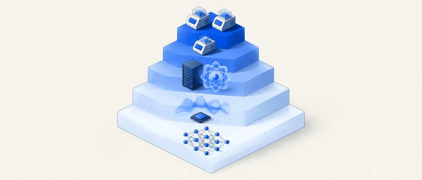
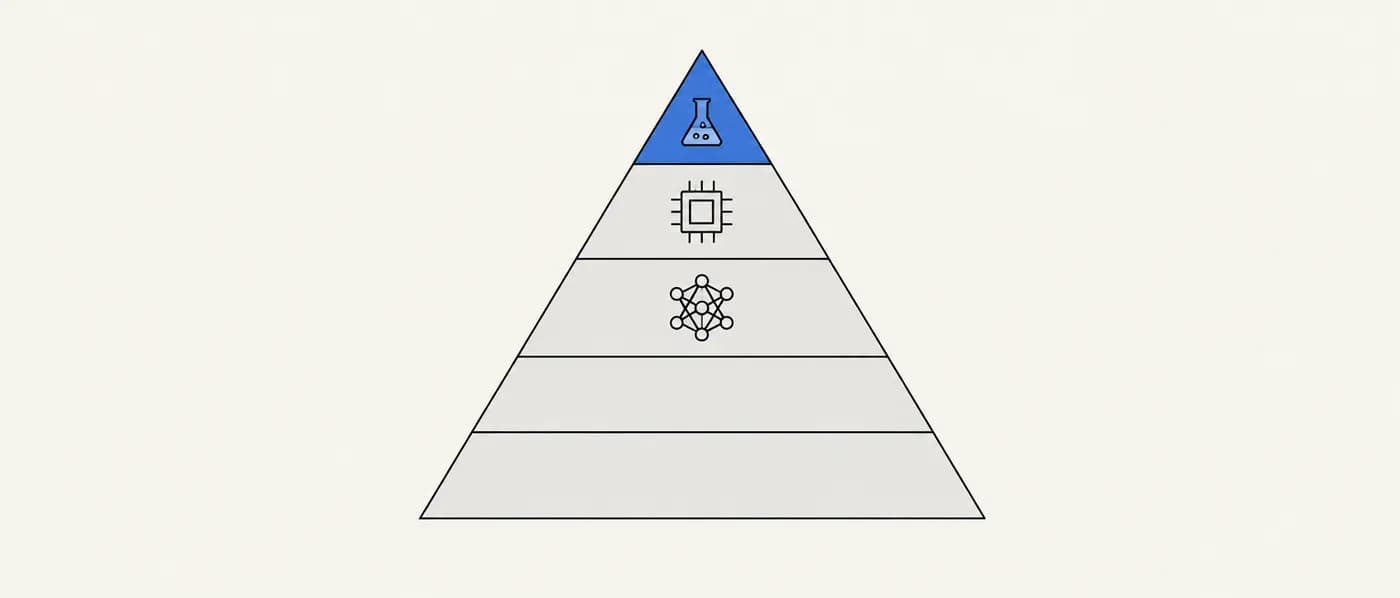
A practical ordering for materials properties is: repeated, independent experiments on well-characterised samples; a single experimental report; higher-level electronic-structure theory (for example hybrid functionals such as HSE06, meta-GGA potentials such as TB-mBJ, or many-body methods such as GW); standard semi-local DFT (GGA functionals such as PBE, often with empirical corrections); and machine-learning predictions trained on one of the tiers above. The ordering is a default, not a law — a careful calculation can beat a poorly characterised measurement — but it is the right starting assumption.
The point is not to discard lower tiers. Standard DFT and ML make it possible to screen millions of compounds that will never be measured. The point is to know which tier each number comes from, so you can choose the right amount of confidence and the right next step.
Why it matters for R&D decisions
A single R&D document often mixes measured conductivities, DFT stabilities and ML-predicted band gaps in the same table without saying which is which. Readers then treat them as equally reliable. That is how a PBE-level gap ends up in a product brief, or a model prediction ends up justifying a synthesis budget. Labelling tiers costs one column in a table and prevents the most common category of overclaiming in materials work.
How to apply it, step by step
- 1Tag every value with its tier
For each number you use, record whether it is measured (and how often), computed at high level, computed at standard DFT, or ML-predicted. Add the method name: ‘PBE’, ‘HSE06’, ‘EIS at 25 °C’, ‘graph neural network trained on PBE energies’.
- 2Know each tier’s characteristic bias
Standard GGA functionals systematically underestimate band gaps. ML models inherit the biases of their training tier and add their own error on top. Experiments depend on sample quality, phase purity and conditions such as temperature. A tier tells you which direction the error is likely to go.
- 3Prefer the highest tier available for the decision property
If a measured value exists for the property that drives your decision, use it and cite it. Use computed values to fill gaps, not to overrule good measurements.
- 4Escalate tiers only where the decision is close
Use cheap tiers to screen broadly. Spend higher-level calculations or experiments on the candidates whose fate depends on a value near your threshold.
- 5Never let a lower tier silently replace a higher one
When merging datasets, keep the tier label with each row. A merged column that mixes measured and predicted values without a flag is a trap for every later user.
Worked examples
Silicon’s band gap: one material, four answers
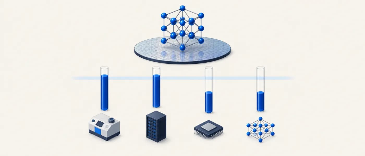
You are building a screen for photovoltaic absorbers and use silicon as a sanity check.
- 01Experiment: silicon has an indirect band gap of about 1.12 eV at room temperature.
- 02Higher-level theory: hybrid (HSE06) and TB-mBJ calculations give values close to the measured gap, roughly 1.1–1.2 eV.
- 03Standard DFT: PBE gives roughly 0.6 eV — about half the measured value, the well-known semi-local band gap underestimation.
- 04ML: a model trained on PBE gaps will, at best, reproduce the PBE value of about 0.6 eV for silicon, because that is what it was taught.
- 05Conclusion: if your screen keeps absorbers with gaps of 1.0–1.8 eV using PBE or PBE-trained ML values, it will wrongly reject silicon.
An ML prediction cannot be more accurate than the tier it was trained on, with respect to that tier’s systematic bias.
Labelling a candidate table for a steering meeting

A shortlist of three solid-electrolyte candidates is going to a steering committee. The table has columns for stability, conductivity and electrochemical window. All numbers below are hypothetical.
- 01Stability (energy above hull): standard DFT, two sources — tier 4, cross-checked.
- 02Room-temperature conductivity: candidate A measured by EIS in two independent papers (tier 1); candidate B measured once (tier 2); candidate C predicted from a model of migration barriers (tier 5).
- 03Electrochemical window: computed from DFT phase equilibria for all three (tier 4).
- 04Add a ‘tier’ marker next to each cell and a one-line legend under the table.
The tier label changes the decision even when the numbers stay the same.
When a measurement is the weaker evidence
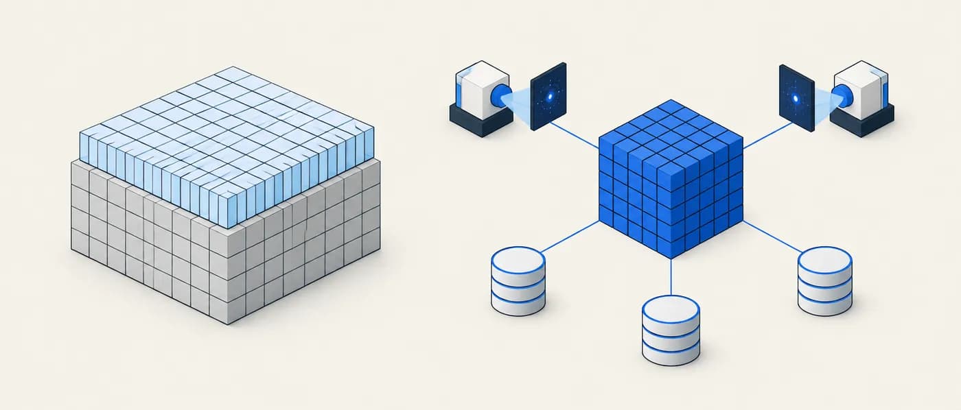
A thin-film paper reports a lattice parameter for a compound that disagrees with three DFT databases by 3%, while bulk diffraction data from two other groups agree with DFT to within 1%.
- 01Classify: thin-film single report (tier 2, with known substrate strain effects) vs repeated bulk measurements (tier 1) and standard DFT (tier 4).
- 02Note that epitaxial strain can change in-plane lattice parameters of thin films.
- 03Prefer the repeated bulk measurements for the bulk property; treat the thin-film value as describing the strained film.
The hierarchy is a default ordering; conditions and sample quality can move a value up or down.
Tiers of materials evidence
| Tier | Examples | Strength | Typical weakness |
|---|---|---|---|
| 1 · Repeated experiment | Independent groups, characterised samples | Directly observes the property | Slow and costly; conditions vary |
| 2 · Single experiment | One paper or one lab measurement | Real sample, real conditions | Sample quality, phase purity, unrepeated |
| 3 · Higher-level theory | Hybrid functionals (HSE06), TB-mBJ, GW, coupled cluster for molecules | Smaller systematic errors for many properties | Expensive; limited coverage |
| 4 · Standard DFT | GGA (PBE), with or without empirical corrections | Consistent, covers millions of compounds | Systematic biases, e.g. band gaps too small |
| 5 · ML prediction | Models trained on tiers 1–4 | Instant, can cover unseen compositions | Inherits training bias; larger error outside training data |
When to use it — and when not to
- Whenever numbers from different origins appear in the same table, chart or decision document.
- When merging datasets from experiment, DFT and ML into one analysis.
- When deciding which candidates deserve expensive calculations or experiments.
- Before quoting a property in marketing, sales or investor material.
- As a reason to ignore a well-designed calculation because a poor-quality measurement exists — judge sample quality and conditions, not just the tier name.
- As a ranking of scientific merit: lower tiers are indispensable for breadth, and the hierarchy is about evidential weight for a specific value.
Common mistakes
Applying it in Lattice Graph
LatticeGraph keeps row-level provenance, so each value carries its source and, where the source records it, its method. Use that to tier your evidence before it goes into your evidence pack.
- 01For each property in your shortlist, open provenance and note whether each value is experimental, computed or predicted, and with which method.
- 02Prefer experimental sources (for example crystal structures from COD, thermochemistry from NIST) where they cover your decision property.
- 03Use cross-source confidence within a tier (DFT vs DFT) rather than across tiers.
- 04In the evidence pack, label each claim as measured, computed or predicted.
Frequently asked questions
Is higher-level theory always better than standard DFT?
For band gaps and many electronic properties, hybrid and many-body methods are usually closer to experiment than GGA. For other properties the gain varies, and higher-level methods have their own errors. Treat the ordering as a default and check benchmarks for your property.
Where do empirically corrected DFT energies fit?
Still in the standard-DFT tier, but with smaller systematic error for the compound classes the correction was fitted on. Corrections can introduce offsets between databases that use different schemes.
How should I report a value when only ML predictions exist?
Report it as predicted, give the model’s benchmark error for that property, and state whether the material is similar to the model’s training data.
References & further reading
- [1]Perdew, J. P., Burke, K., & Ernzerhof, M. (1996). Generalized gradient approximation made simple. Physical Review Letters, 77, 3865–3868.The PBE functional used by most large computed databases.
- [2]Heyd, J., Scuseria, G. E., & Ernzerhof, M. (2003). Hybrid functionals based on a screened Coulomb potential. The Journal of Chemical Physics, 118, 8207–8215.The HSE hybrid functional, a common higher-level choice for band gaps.
- [3]Tran, F., & Blaha, P. (2009). Accurate band gaps of semiconductors and insulators with a semilocal exchange-correlation potential. Physical Review Letters, 102, 226401.The TB-mBJ potential used by JARVIS-DFT for improved band gaps.
- [4]Borlido, P., Aull, T., Huran, A. W., Tran, F., Marques, M. A. L., & Botti, S. (2019). Large-scale benchmark of exchange–correlation functionals for the determination of electronic band gaps of solids. Journal of Chemical Theory and Computation, 15, 5069–5079.Quantifies how different functionals compare with experimental band gaps.